Best Unified Data Lakehouse Platforms with Transparent Pricing and No Hidden Compute Costs
A procurement framework for evaluating unified data lakehouse platforms on pricing transparency: seven testable criteria, billing mechanics, TCO worksheet and acceptance checklist.
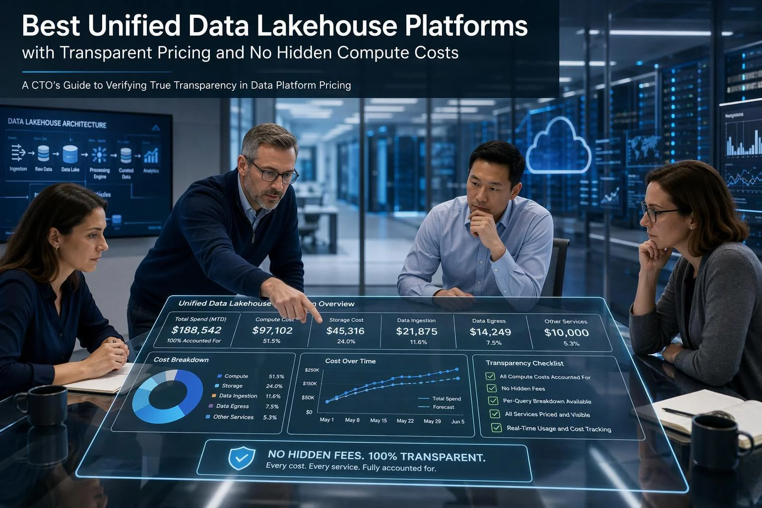
Transparent pricing is not a vendor attribute you can look up on a pricing page. It is a set of testable properties you have to verify against each platform's billing mechanics, because the cost that surprises buyers is almost never storage — it is compute, and compute is the line item that scales with your own query volume rather than with your provisioning choices.
This guide is written for the people who sign the multi-year commitment: the CTO or VP of engineering who owns the architecture, the data architect who owns the workload, and the procurement or finance partner who owns the forecast. It compares Databricks, Snowflake, BigQuery, Amazon Athena and EMR, Microsoft Fabric, ClickHouse-based services, and self-managed open source strictly on how legible their billing is, using vendor documentation rather than performance claims. The method runs in four stages: characterize your own workload, score each platform against seven transparency criteria, screen for red flags, then gate signature on an acceptance test.
Why "No Hidden Compute Costs" Is Harder Than It Sounds
Hidden compute cost rarely means a vendor is concealing a rate. It means a cost driver is billed but not modeled by the buyer: a per-second rate with a minimum charge, a cluster that starts because queries queued, a serverless premium applied to a feature you assumed was included, a maintenance job that consumes billable compute on a schedule you did not set, or egress on a data path nobody mapped.
A useful working definition: a platform is transparent to the extent that every cost driver is (a) documented, (b) attributable to a workload, user or team in billing data, and (c) controllable by the customer through configuration. Fail any one of the three and the cost is effectively hidden even when the rate card is public — documented but unattributable costs cannot be charged back, and attributable but uncontrollable costs cannot be capped.
Storage and compute are usually separable, and that separation is where the surprises live. When the two are coupled — scan-based pricing being the clearest case — the cost of a query depends on how the data is physically stored, so a storage decision silently becomes a compute decision.
Start With a Needs Assessment Before You Compare Vendors
Transparency criteria only matter relative to the cost drivers you will actually hit, so characterize your workload before you open a single pricing page. The output of this step is the input to the scoring framework in the next section: it tells you which of the seven criteria to weight heavily and which to treat as a formality.
Workload characteristic | What to record | Why it shifts which cost drivers dominate |
|---|---|---|
Workload mix | Share of BI/SQL, batch ETL, streaming, ML/feature engineering, ad-hoc analysis | Concurrency-sensitive pricing punishes BI; scan-based pricing punishes wide batch reads |
Concurrency profile | Peak concurrent users and queries, burstiness, business-hours vs. 24/7 | Drives multi-cluster and autoscaling behavior, the most common source of bill shock |
Data volume and scan patterns | Columnar vs. raw text, partitioning, compression ratio | Determines whether per-terabyte scanning is cheap or ruinous |
Ingestion cadence | Batch windows, streaming inserts, change-data-capture volume | Streaming and frequent small writes often carry separate pricing surfaces |
Retention and tiering | Hot/cold split, archival age, regulatory retention | Storage tier design and restore costs |
Regions and cloud topology | Multi-cloud, cross-region replication, BI tools outside the cloud | Egress and cross-region transfer become material line items |
Governance and isolation | Tenant isolation, residency, audit requirements | May force dedicated compute, removing shared-capacity savings |
Operating model | Who runs the platform, who owns the cost number | Determines whether unattributed cost is a real risk or a rounding error |
Fill this in with measured numbers where you have them — query concurrency from your existing warehouse logs, scan volume from your current bill — and with labeled estimates where you do not. A needs assessment built entirely on guesses will produce a scoring model that weights the wrong criteria.
The Transparency Evaluation Framework: Seven Testable Criteria
Score each platform 0–3 on the seven criteria below, weighting them by your needs-assessment output. This is a procurement-practice framework, not a benchmark; validate every score against the vendor's own documentation and a trial.
Snowflake's published credit-per-hour rates for Gen1 standard warehouses, by size. These are list rates per cluster per full hour of running; actual billing is per second with a 60-second minimum each time a warehouse starts. Rates are credits, not dollars — the dollar value of a credit depends on edition and contract.
Criterion 1: Published Unit Pricing and Billing Granularity
Granularity matters more than the headline rate. Snowflake publishes a credit-per-hour table by warehouse size, from X-Small at 1 credit/hour to 6X-Large at 512 credits/hour, and bills per second with a 60-second minimum each time a warehouse starts — so a 10-second query on a just-started warehouse still pays a full minute. Verify by finding the unit table, confirming the interval and minimum, then pricing one representative short query and one long query.
Criterion 2: Cost Attribution and Billing Data Export
Transparency requires reconciling bills to workloads. Databricks exposes billing usage through system tables, including a list_prices table of list prices over time per SKU that can be joined to usage, and documents that classic-compute TCO requires reconciling platform DBU costs with cloud infrastructure costs because customers manage compute directly with the provider. Verify by asking for a native export at job and user granularity, and whether list and effective prices are both present.
Criterion 3: Compute-Scaling Mechanics Disclosed
Autoscaling is the most common source of bill shock because query volume, not provisioning, drives spend. Snowflake's multi-cluster warehouses make the trade-off explicit: the Standard policy favors starting a cluster when queries queue, while Economy starts one only if it estimates at least six minutes of work and shuts down clusters with less than six minutes of work remaining. Verify that the vendor documents its policies and their billing consequences, and whether you can cap maximum clusters.
Criterion 4: Serverless and Managed-Feature Premiums Itemized
Serverless is convenient and usually priced at a premium, so the premium must be visible per feature. Databricks describes serverless compute as a versionless managed product and lists serverless SKUs separately from classic compute — on the Azure Databricks price list, Interactive Serverless, Automated Serverless and Serverless SQL are distinct DBU-hour lines. Verify a published SKU rate for each managed feature you plan to use, and that it appears as its own billing line.
Criterion 5: Background and Maintenance Compute Disclosed
Compaction, clustering, vacuum, and materialized-view or streaming-table refresh can consume billable compute, and whether they do is a transparency test. Databricks states that materialized view and streaming table creation and updates are charged at DLT Serverless rates and billed using Automated Serverless SKUs. Verify by asking the vendor to enumerate every background operation that bills, its SKU, and whether you can schedule, throttle or disable it.
Criterion 6: Data Movement and Egress Pricing Documented
Egress and cross-region transfer is a classic hidden cost for multi-cloud and external-BI architectures. Athena illustrates the layering: there is no additional Athena storage charge for querying S3, but standard S3 rates apply for storage, requests and data transfer, and query results are written to S3 and billed at S3 rates — so the Athena rate is only part of the bill. Verify a published rate for every hop from source to lakehouse to BI tool to archive.
Criterion 7: Commitment and Discount Structure Disclosed
Commitments improve unit economics but reduce transparency when the interaction between commitment, on-demand rates and unused capacity is undocumented. Databricks offers pay-as-you-go billing at per-second granularity and committed-use contracts with discounts and cross-cloud flexibility, but directs buyers to sales for details — score that gap accordingly. Verify the contract's definition of a unit, how overage bills, whether unused commitment rolls over, and whether discounts reach serverless SKUs.
Platform-by-Platform Transparency Comparison
The table below scores transparency mechanics, not price levels or performance, and list prices change — re-verify against current vendor pages before you rely on any cell.
BigQuery capacity pricing per slot-hour, list rate versus one- and three-year committed-use discounts (Standard edition). Billed per second with a 1-minute minimum unless Fluid scaling is opted into. Values are USD per slot-hour.
Databricks
Databricks is strongest on attribution: system tables, the list_prices table, and documented cost-monitoring dashboards give a buyer real reconciliation tooling, and serverless versus classic compute is published as separate SKUs. The gaps are commitment transparency, where discount mechanics sit behind a sales conversation, and classic-compute TCO, which requires joining DBU costs to cloud infrastructure data such as AWS CUR. On Azure, Databricks is a first-party service with unified billing and support by Microsoft, and Azure Databricks pricing is set by Microsoft.
Snowflake
Snowflake publishes credit tables and per-second billing mechanics with unusual clarity, and documents its multi-cluster scaling policies and their credit consequences. The challenge is that concurrency scaling, serverless features and cloud-services credits are separate billing surfaces you must model together. One easy-to-miss mechanic: cloud services usage is billed only for the amount exceeding 10% of daily warehouse compute, calculated daily in UTC — documented, but invisible unless you read the compute-cost page.
Google BigQuery
BigQuery offers two compute models: on-demand, charged per TiB processed, and capacity, charged per slot-hour with autoscaling and optional one- or three-year commitments. The structure is transparent, but the buyer must choose and model the right model for their workload. Storage bills by logical versus physical bytes with active and long-term rates, and several features have separate pricing surfaces — streaming inserts, for example, are listed at $0.01 per 200 mebibyte — so the compute rate alone does not describe the bill.
Amazon Athena and Amazon EMR
Athena prices SQL by data scanned or by DPU-hour capacity reservation, and its pricing page walks through a worked example where GZIP compression and Parquet conversion cut a 3 TB scan from $15 to $1.25. EMR bills per second with a one-minute minimum, but the EMR rate is added to EC2 and EBS charges, so the platform line is a fraction of the bill. Both are transparent at the unit level and opaque at the total level until you model S3, EC2 and EBS yourself.
Microsoft Fabric
Fabric sells capacity units on a published SKU ladder from F2 to F8192, with pay-as-you-go or reservation pricing, OneLake hot/cool/cold storage tiers, and an opt-in capacity overage mechanism that lets mission-critical capacities pay for excess consumption with an optional 24-hour limit. Two gaps matter: displayed prices are estimates converted from USD and vary by agreement, and Spark autoscale bills at standard regional pay-as-you-go CU-hour rates that reservation discounts do not cover.
ClickHouse-Based Platforms
ClickHouse Cloud meters compute per minute in 8 GB RAM increments and shows usage per service by metered dimension in its console, per the billing overview. Third-party comparisons that frame ClickHouse as the transparent alternative to per-TB warehouses are vendor-adjacent marketing, so treat them as positioning rather than evidence. The test for any specific managed offering is whether it publishes compute and storage unit rates and whether background merges consume billable compute.
Self-Managed Open Source
Self-managed open source inverts the transparency profile. Every dollar is a cloud infrastructure line item you can see and control — compute, storage, egress — but no vendor publishes a platform unit price, because the platform layer is your engineers' time. The hidden costs are operational: cluster management, tuning, compaction and vacuum jobs your team must schedule and staff. Use it as the baseline against which every managed premium is judged, and price engineering hours explicitly rather than treating them as free.
Red Flags and Deal-Breakers
Red flags are warning signs that justify deeper diligence. Deal-breakers are conditions that should end the evaluation regardless of how good the demo looked. Keeping the two apart prevents a slow, expensive procurement from turning a caution into a veto — or the reverse.
Red flags worth escalating:
Pricing pages that render as
$-/unitplaceholders, so list prices only exist inside a sales conversation. The Azure Databricks and Microsoft Fabric pages both display this pattern, and both note that displayed prices are estimates rather than quotes.Committed-use discounts described only as "contact us," with no published mechanics for how commitment, on-demand rates and unused capacity interact.
Serverless features with no published SKU rate, or rates that appear only as a footnote on a product page.
No native billing export at workload, job or user granularity.
Background maintenance compute that cannot be scheduled, throttled or capped.
Egress rates that live only on the cloud provider's page, with no platform-level summary of which data paths incur them.
Deal-breakers:
No mechanism to cap spend or alert on it before the invoice arrives.
No way to attribute cost to teams, projects or cost centers, which makes chargeback and budget ownership impossible.
Contract terms that forfeit unused commitment with no rollover and no documented overage rate.
Billing granularity that makes your dominant workload uneconomical, with no alternative pricing model offered. A short-query BI estate facing a 60-second minimum on every warehouse start is the clearest case.
One caution on the last item: a granularity mismatch is only a deal-breaker if the vendor cannot offer a different model. BigQuery, for example, documents both on-demand per-TiB pricing and capacity pricing per slot-hour, so a workload that fits one model badly may fit the other well. Score the mismatch against the alternatives on the table, not against an ideal.
Building the TCO Worksheet
The seven criteria tell you what to ask; the worksheet tells you what the answers cost. Build it in four layers so a missing answer shows up as a blank line rather than an invisible assumption.
Athena's own worked example: the same single-column query over a 3 TB dataset, priced at $5 per TB scanned. Compression and columnar conversion change how much data the engine must read, and therefore the bill — the rate itself never moves. Values are USD per query.
Layer 1 — Platform units. For every SKU in your proposed architecture, multiply the published unit rate by projected units: classic compute hours, serverless DBU-hours or credit-hours, SQL warehouse hours, storage GB-months, and data transfer. Include background maintenance SKUs explicitly; if the vendor cannot name them, leave the line blank and flag it.
Layer 2 — Cloud infrastructure. Where compute is billed through the cloud provider — Databricks classic compute, EMR on EC2, self-managed anything — add EC2, EBS, S3 and egress lines. Databricks states that classic-compute TCO requires reconciling platform DBU costs with cloud infrastructure costs because customers manage compute directly with the provider, and its cost-unification guidance describes joining AWS CUR or Azure Cost Management exports to system tables.
Layer 3 — Operations. Price engineering FTE time for platform management, maintenance and cost governance. This is the line most worksheets omit and the one that most often decides self-managed versus managed.
Layer 4 — Commitment. Model on-demand against committed pricing, then add the cost of unused commitment under your realistic utilization range.
Illustrative example (an inference, not observed data). Suppose a team scans 200 TB per month for BI and runs 400 hours of batch ETL. On a scan-priced engine at $5/TB, the BI line is roughly $1,000 per month and scales linearly with how much data analysts touch — a badly partitioned dashboard doubles it. On a compute-priced engine, the same BI volume might cost far less per query but carries a fixed floor per warehouse start, so a thousand ten-second queries can cost more than a hundred long ones. Neither shape is inherently cheaper; they fail in different directions. That is why the worksheet must be run three times: current workload, 2× growth, and peak/burst. The scenario that breaks your budget is usually the third.
Negotiation Questions to Ask Vendors
Ask these in writing and attach the answers to the contract as a pricing exhibit. Verbal assurances about billing behavior do not survive a renewal conversation.
Unit pricing and granularity
Show the published SKU rate for every feature in our proposed architecture, including serverless and background maintenance.
How do you bill a query that runs 10 seconds on a warehouse that just started? What is the minimum billing interval?
Are list prices and effective discounted prices both visible in billing data?
Attribution
Can we export billing data at job, user and team granularity, and in what format and cadence?
Does the export include list prices over time so we can reconcile historical charges?
Scaling
What scaling policies do you offer, and how does each translate into billed units under the same query load?
Can we cap maximum clusters, maximum concurrency or maximum spend, and what happens when the cap is hit?
Serverless and maintenance
Which background operations consume billable compute, at what SKU, and can we schedule, throttle or disable each one?
Do materialized view and streaming table refreshes bill at serverless rates?
Data movement
How do you price egress to our BI tool, to our archive region, and across clouds?
Which data paths incur cloud-provider transfer charges that do not appear on your invoice?
Commitment
What is the contract's definition of a unit, how is overage billed, and does unused commitment roll over or expire?
Do committed-use discounts apply to serverless SKUs or only to classic compute?
Acceptance Checklist Before You Sign
Gate signature on binary pass/fail items. A partial answer is a fail until it is documented in writing.
Published unit price exists for every SKU in the proposed architecture.
Billing interval and any minimum charge are documented, and you have computed the cost of a representative short query and a representative long query.
Native billing export is available at workload, job or user granularity, including list prices over time.
Scaling policy options are documented with their billing consequences, and customer-set caps exist.
Serverless and managed-feature SKU rates are published and appear as distinct billing lines.
Every background operation that consumes billable compute is enumerated, with its SKU and whether it can be scheduled or disabled.
Egress and cross-region transfer rates are published for every data path in your architecture.
Commitment, overage and forfeiture terms are in writing, including whether discounts reach serverless SKUs.
A pilot reproduces the TCO worksheet within an agreed tolerance.
The pilot tolerance is a procurement-practice recommendation, not a vendor-published standard. A band of roughly ±15% is a reasonable starting point for negotiation; tighten it for steady workloads and widen it for bursty ones where a single month is not a representative sample. Run the pilot long enough to include a month-end close and a peak concurrency event, because those are the periods where scaling and maintenance charges concentrate.
Where Singdata Fits in This Evaluation
Singdata Lakehouse is worth scoring against the same seven criteria, and its architecture speaks most directly to Criteria 3, 4 and 5. Its single-engine design consolidates Spark, Flink and data-warehouse workloads into one engine, which reduces the number of separately billed compute surfaces a buyer has to model — fewer scaling policies, fewer serverless SKUs, fewer maintenance jobs billed on their own line. That is a structural argument about billing surface area, not a price claim.
Singdata reports up to 4× faster performance than Snowflake, up to 10× faster than Spark, roughly 50% lower total cost of operation and about 80% reduction in architecture complexity. Treat these as vendor-reported claims to validate in your own pilot, exactly as you would treat any competitor's headline numbers. Ask for the published unit rates behind them, run the TCO worksheet on your own workload, and confirm which operations consume billable compute.
If Singdata survives that screen, a pricing discussion through Singdata's site is the natural next step. If it does not, you have lost an afternoon and gained a defensible comparison.
FAQ
What counts as a "hidden" compute cost in a lakehouse?
A cost driver that is billed but neither attributable to a workload in your billing data nor controllable through configuration. The usual suspects are concurrency-driven scaling, serverless premiums, background maintenance jobs and egress.
Is per-second billing always cheaper than per-minute?
No. A per-second rate with a 60-second minimum behaves like per-minute billing for short queries. Snowflake documents per-second billing with a 60-second minimum each time a warehouse starts, and BigQuery's capacity pricing is billed per second with a 1-minute minimum unless you opt into Fluid scaling. For bursty short-query workloads, the minimum, not the rate, sets the bill.
Why do Databricks TCO calculations need cloud cost data?
Because classic compute is billed through your cloud provider. Databricks platform DBU costs and infrastructure costs are separate data sources that must be reconciled — Databricks documents this explicitly and publishes a solution for joining them.
Does BigQuery's on-demand or capacity model offer more transparency?
Both are documented. On-demand per-TiB pricing is simpler to forecast for variable workloads; capacity per slot-hour is more predictable for steady high-volume workloads. The right choice depends on your needs assessment, not on which model sounds more transparent.
Are committed-use discounts less transparent?
They can be, when overage and forfeiture terms are not documented. Require the definition of a unit, the overage rate and the treatment of unused commitment in writing before signing.
How do I compare a scan-based platform to a compute-based platform?
Run both through the TCO worksheet for the same workload, including storage and egress, across current, 2× growth and peak scenarios. Compare the shapes of the cost curves, not just the monthly totals.
Return to the acceptance checklist before you sign; every question above maps to an item on it.