
High-Concurrency Logistics and E-Commerce Lakehouse Use Cases
A practical guide to high-concurrency lakehouse design for logistics and e-commerce: why mixed workloads degrade, how to separate request-rate from interference, freshness targets per decision, labeled use-case patterns, a peak-event load-test protocol, and silent-failure detection.
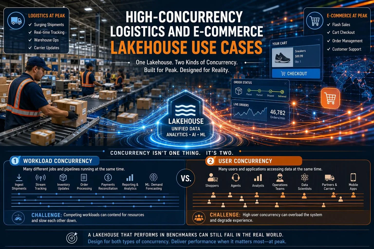
A lakehouse can post excellent numbers on a single-workload benchmark and still miss its service targets on a Tuesday afternoon in November. The difference is not the engine's raw speed. It is what happens when a change-data-capture (CDC) job streaming shipment scans, a dashboard refresh serving 400 dispatch planners, and an analyst running an ad-hoc join against eighteen months of order history all hit the same tables within the same ninety seconds. Each workload is reasonable in isolation. Together they contend for the same commit path, the same compute pool, and the same metadata.
This guide separates two things that the word "concurrency" hides. The first is request rate: how many queries, sessions, or ingestion streams arrive per unit time. The second is interference: how much concurrent work slows other work down through shared resources. A platform can be strong on the first and weak on the second, and most vendor concurrency claims describe only the first.
The scope is logistics operations and e-commerce commerce workloads running on one lakehouse: shipment tracking, inventory promise, dispatch, delivery SLA monitoring, order and payment events, catalog state, promotion performance, and session analytics. The sections that follow move through why mixed workloads degrade, how to measure each kind of concurrency, how to set freshness targets from the decision rather than the pipeline, labeled design patterns for logistics and commerce, a peak-event load-test protocol with pass/fail criteria, and the silent failures that produce no error at all.
One convention applies throughout. Freshness targets, workload mixes, and use-case patterns here are engineering judgment or explicitly illustrative designs, not observed benchmarks. Where a vendor reports a performance or concurrency figure, it is presented as a claim to reproduce in your own environment, not as an established property of the category.
Why a Lakehouse Degrades Under Mixed Workloads
The usual explanation blames the heaviest workload. That is rarely the mechanism. Degradation under mixed load comes from four shared surfaces that behave well when only one workload touches them and badly when several do at once.
Commit coordination. Open table formats built on optimistic concurrency, Apache Iceberg among them, assume that a writer operates alone and only discovers otherwise at commit time. As the Iceberg reliability documentation describes it, each writer produces new table metadata and attempts to commit by atomically swapping the new metadata file for the existing one. If the swap fails because another writer committed first, the failed writer retries by building a new metadata tree against the new current table state. Iceberg reduces the cost of those retries by structuring changes so work can be reused, for example by writing a new manifest for appended files rather than rewriting the manifest on every attempt. But reuse is not free, and the number of writers competing for the same table is the variable that matters.
Write frequency. A CDC job that commits every five seconds and a CDC job that commits every five minutes put very different pressure on that commit path. High-frequency micro-batches multiply the number of commit attempts, and each conflict costs a retry cycle. The same table receiving a compaction job, a late-arriving-data append, and a streaming upsert is a three-way contention point that no single-workload test exercises.
File layout and metadata volume. Iceberg tracks the complete list of data files in each snapshot using a persistent tree structure, which is what makes planning an O(1) metadata read rather than a directory listing. That advantage depends on the tree staying reasonably sized. A table that accumulates millions of small files from frequent small commits forces every reader to plan across a larger manifest set, and the read cost that looked trivial in a benchmark becomes visible when fifty dashboards plan against the same table simultaneously.
Compute contention. Even with storage and metadata healthy, a fixed compute pool divides its capacity among whatever is running. A dashboard refresh that scans a wide fact table will starve an ingestion job sharing the same pool, and the ingestion job's lag then propagates into every downstream freshness guarantee.
The consequence is that "each workload is fast alone" and "the combination is slow" are both true and neither predicts the other. A benchmark that runs one query shape against a tuned table, with no concurrent writer and no compaction running, measures the engine. It does not measure the system under the conditions that actually cause incidents. Vendor concurrency figures, including those published for real-time lakehouse engines, are worth reading as claims about a tested configuration; the only reliable evidence is a mixed-workload run against your own tables, your own commit cadence, and your own query shapes.
Two Kinds of Concurrency: Request Rate vs. Mixed-Workload Interference
Treat these as separate measurements with separate remedies, because a fix for one routinely does nothing for the other.
Request-rate concurrency is a queueing property. It asks how many simultaneous requests the system can admit before wait time dominates service time. Measure it with queue time (the interval between submission and the start of execution) and with latency percentiles at fixed arrival rates, not with averages. A p50 that holds steady while p95 climbs is the signature of a queue forming. Concurrent session counts and queue depth are the leading indicators; they move before the latency percentiles do.
Interference concurrency is a contention property. It asks how much one workload's progress degrades another's when they overlap. Measure it with commit-conflict counts and retry counts per table per hour, with the ratio of retried to committed transactions, and with cross-workload latency correlation: does dashboard p95 rise specifically during the ingestion window, and does ingestion lag rise specifically during the morning reporting peak? If the two curves move together, you have interference. If latency rises uniformly across all workloads regardless of what else is running, you have a request-rate or capacity problem.
A practical attribution test: run the suspect workload alone at its production rate and record latency. Then run it alongside the other workloads at their production rates. If latency is acceptable alone and unacceptable together, and commit retries or shared-pool saturation rise in the second run, the cause is interference. If latency is already unacceptable alone, the workload needs tuning or more capacity and no amount of isolation will fix it.
The distinction matters because the common scaling remedy addresses only the first kind. Snowflake's documentation is unusually direct about this. Multi-cluster warehouses are described as best utilized for scaling resources to improve concurrency for users and queries, and explicitly as not as beneficial for improving the performance of slow-running queries or data loading; for those operations, resizing the warehouse is the recommended lever. The warehouse overview adds that resizing can enable limited scaling for query concurrency and queuing but is primarily intended for improving query performance. Amazon Redshift's concurrency scaling similarly routes eligible queries to additional clusters to maintain consistent response times under high request volume, with documented eligibility limits.
Read those statements as scope definitions, not criticisms. Adding clusters absorbs more simultaneous readers; it does not resolve two writers fighting over the same Iceberg table's commit path, and it does not make a compaction job stop competing with a streaming upsert. If your incident is retry storms on three hot tables, buy isolation and commit-cadence discipline, not more clusters.
Freshness Targets per Operational Decision
Most freshness requirements are inherited from what the pipeline happens to deliver, then defended as if they were business needs. Derive the target from the decision instead. Two inputs determine it: how often the decision is actually made, and what it costs to make it on stale data.
A decision made once per shift does not benefit from ten-second data. A decision made continuously, where each minute of staleness produces a wrong action, does. The target should sit just inside the decision cadence, with enough margin that the data is reliably there when the decision point arrives. Anything fresher than that consumes ingestion capacity, commit bandwidth, and storage churn for no operational return.
The table below is a design-target framework, not measured data. The targets are engineering judgment for a mid-size logistics and commerce operator; treat them as starting points to justify or reject against your own cost-of-staleness estimates.
Decision | Cadence | Illustrative target | Why this target | Where tighter has no payoff |
|---|---|---|---|---|
Inventory promise at checkout | Continuous, per request | Seconds; served from an operational store, not the lakehouse | A stale promise oversells stock and creates a cancellation | Sub-second lakehouse freshness; the promise path should not query the lake at all |
Dispatch and route assignment | Per wave, every 15–60 min | Minutes | Assignments are batched to waves; a five-minute-old view is sufficient | Real-time per-second updates during a wave already in progress |
Fraud hold decision | Per order, at authorization | Seconds to low minutes | Holds must resolve before fulfillment commits | Sub-second; the cost of a marginally later hold is small |
Campaign bid adjustment | Every 5–30 min | Minutes | Bid changes need time to take effect in the ad platform anyway | Second-level; platform latency dominates |
Delivery SLA monitoring | Continuous alerting | Minutes for alerting, hourly for trend | Alerts must fire before the SLA breach is unrecoverable | Sub-minute alerting on a 24-hour SLA window |
Executive reporting | Daily or weekly | Hours to a day | The review happens on a schedule | Anything fresher than the meeting |
Settlement and reconciliation | Daily | Next-day completeness | Correctness and completeness matter more than speed | Intraday freshness; settlement runs on closed periods |
Two disciplines keep this table honest. First, write the cost of staleness in the units the business uses — cancelled orders per hour, misallocated dispatch minutes, SLA credits — rather than in pipeline terms. Second, record the target as a service-level objective with a measurement method attached, so that "five minutes" means p95 end-to-end lag measured from source event time to queryable state, not the scheduler interval.
Vendor freshness figures, such as a claim of five-minute freshness across an entire pipeline, describe a vendor's tested configuration. They are useful as an existence proof that the target is achievable and useless as a guarantee for your schema, your commit cadence, and your peak load.
Logistics Use Cases: Data Model, Grain, and Failure Modes
The patterns below are illustrative designs, not descriptions of any named company's production system. Each one names the grain explicitly, because most logistics data defects are grain defects: an event-level table queried as if it were shipment-level, or a stop-level metric averaged as if it were shipment-level.
The problem class is real and documented. The AWS Big Data Blog's account of BigBasket's Iceberg-based lakehouse describes ETL pipelines delivering only day-old (D-1) data, which made near-real-time dashboard analysis impossible, alongside infrastructure that struggled with load rising from 13,000 to over 35,000 transactions for reports and dashboards with more than 1,000 dataset refreshes. That combination — stale data and refresh load growing faster than the platform — is the shape this section addresses.
Shipment tracking events. Model as an append-only event table keyed by shipment and carrier, with event time, observation time, carrier scan code, and location. Grain: one row per carrier event. Concurrency shape: write-heavy, high-frequency CDC or webhook ingestion, with a comparatively light read load from tracking pages. Validation checkpoint: for every open shipment, confirm that the latest observed event time is consistent with the carrier's expected scan cadence for that lane. Failure mode: conflating "nothing happened" with "we did not receive the update." Practitioner guidance on tracking API reliability makes the point directly — a shipment that has not moved is not automatically stale, because international transit, handoffs, weekends, and carrier scanning practices produce legitimate gaps. The monitoring problem is to separate a quiet shipment from a missed update, and that requires per-carrier, per-lane thresholds rather than one global refresh interval.
Inventory promise and allocation. Model as a current-state table at the SKU-location grain, fed by an append-only reservation and release event stream. Grain: one row per SKU per location, with the event stream retained for audit. Concurrency shape: read-heavy at checkout, write-heavy from order and cancellation events; this is the table where interference is most expensive. Validation checkpoint: reconcile the sum of open reservations against the state table on a fixed interval and alert on divergence. Failure mode: a stale read that promises stock already reserved, which surfaces as a cancellation rather than an error.
Dispatch and route assignment. Model at the stop grain, with a shipment-level rollup for reporting. Grain: one row per stop per route plan version. Concurrency shape: bursty reads during wave planning, moderate writes as plans are revised. Validation checkpoint: every shipment in a released plan must appear in exactly one stop, and every stop must have an assigned vehicle and time window. Failure mode: plan versions coexisting without a clear current-version marker, so two planners act on different plans.
Delivery SLA monitoring. Model as a derived table at the shipment grain, computed from promised window, actual delivery event, and exception codes. Grain: one row per shipment, refreshed incrementally. Concurrency shape: continuous incremental writes plus dashboard reads at shift boundaries. Validation checkpoint: compare the count of shipments past their promised window against the operational exception queue; the two must agree. Failure mode: the SLA clock running on ingestion time rather than event time, which silently understates breaches when ingestion lags.
E-Commerce Use Cases: Data Model, Grain, and Failure Modes
Commerce workloads are bursty and read/write-mixed in a way logistics workloads usually are not. The peak shape is documented even if lakehouse behavior at that peak is not. Adobe's 2025 Cyber Monday release, based on Adobe Analytics data covering over 1 trillion visits to U.S. retail sites, reports consumers spending $16 million every minute during the 8 pm to 10 pm peak hours, with $14.25 billion spent online across the day. The same release reports AI traffic to U.S. retail sites up 670% on Cyber Monday, measured by shoppers clicking on a link, while noting the base of users remains modest.
U.S. online retail spend, 2025, Adobe Analytics. Day-level figures (Black Friday, Cyber Monday) and the five-day Cyber Week total (Thanksgiving through Cyber Monday) are shown together; the windows differ, so the five-day bar is not comparable to the single-day bars as a rate. Adobe does not publish order counts, and these are market-level totals, not a per-retailer peak multiplier — measure your own peak ratio against your own baseline.
Those figures describe commerce transaction volume, not lakehouse query load, and should not be read as a benchmark for any data platform. What they establish is the shape of the problem: demand arrives in a narrow window, and the analytical systems behind pricing, inventory, and personalization are asked to answer questions about it while it is still happening.
The patterns below are illustrative designs.
Order and payment event streams. Model as an append-only event table with an explicit event type, an idempotency key, and both event time and ingestion time. Grain: one row per order event, not per order. Concurrency shape: write-heavy and continuous, with a sharp peak during promotions. Validation checkpoint: for a closed period, compare distinct order IDs in the event stream against the order system's count, and compare payment captures against settlement records. Failure mode: duplicate events from at-least-once delivery inflating order counts, which is silent because every individual row is valid.
Inventory and catalog state. Model as a current-state table at the SKU grain with a change history, kept separate from the order event stream. Grain: one row per SKU, with history retained for audit. Concurrency shape: heavy reads from storefront and personalization services, heavy writes from catalog and price updates. Validation checkpoint: catalog price changes must be traceable to an approving event, and the count of active SKUs must match the merchandising system. Failure mode: catalog and inventory updated by different pipelines with different commit cadences, producing a window where a product is purchasable at a price that no longer exists.
Campaign and promotion performance. Model as an incremental aggregate at the campaign-by-hour grain, rolled up to campaign-by-day. Grain: one row per campaign per hour. Concurrency shape: read-heavy dashboards during the campaign, with continuous writes from the event stream. Validation checkpoint: hourly aggregates must sum to the daily total for the same campaign, and both must reconcile to the order event stream. Failure mode: late-arriving events landing after the hourly aggregate closed, so the dashboard and the settlement report disagree permanently.
Customer and session analytics. Model at the session grain, with a customer-level rollup. Grain: one row per session, identified by a session key that survives client retries. Concurrency shape: very high write volume during peaks, with analytical reads that are tolerant of a few minutes of lag. Validation checkpoint: session counts must not exceed request counts from the edge logs, and sessions must not span implausible durations. Failure mode: session keys regenerated on retry, splitting one visit into several and inflating conversion denominators.
Peak-Event Load-Test Protocol with Pass/Fail Criteria
A benchmark run and a peak-event load test answer different questions. A benchmark asks how fast one workload finishes on a tuned system; a load test asks whether the whole platform holds its service levels when ingestion, dashboard refresh, and ad-hoc analysis arrive together and keep arriving. The protocol below is a reusable template, not a set of measured results. Every threshold in it is one you set from your own service-level objectives, and every vendor concurrency figure you have read is a claim to reproduce in your own environment rather than a substitute for running this.
Run the test against a production-shaped copy of the platform: the same table formats, the same partitioning, the same compaction and retention settings, and a data volume at least as large as the peak-season table sizes you expect. A test on a small, freshly written table will understate commit-conflict retries and metadata planning cost, which are exactly the behaviors the test exists to expose.
Workload mix. Define four concurrent streams and hold their ratios fixed across runs so results stay comparable. Ingestion: replay a captured CDC or event stream at the peak rate you expect, preserving the original inter-arrival timing rather than smoothing it. Dashboard refresh: run the actual scheduled reports at their real cadence, including the ones that scan wide date ranges. Ad-hoc analysis: replay a recorded query log from analysts, including the expensive outliers, since those are the queries most likely to collide with ingestion commits. Interactive point lookups: the operational queries that serve customer-facing screens, which have the tightest latency budget and the least tolerance for queueing.
Ramp profile. Start at a documented baseline, hold it for a stabilization window, then ramp to peak over a defined interval rather than stepping instantly. A gradual ramp shows where the system begins to degrade; an instant step mostly shows whether it survives the first minute. Hold peak for longer than your longest realistic burst — a flash sale, a carrier outage that queues scans, a promotion launch — and then ramp down while continuing to measure, because recovery behavior matters as much as peak behavior.
Metrics to capture. Record latency at p50, p95, and p99 separately for each workload stream, not as a single blended figure; a blended average hides the dashboard that went from two seconds to forty. Capture queue time separately from execution time, since queueing is the signature of request-rate saturation while execution time is where interference shows. Capture commit-conflict counts and retry counts per table, freshness lag measured as the gap between event time and query-visible time, error and abort rates, and the count of queries that failed outright rather than ran slowly.
Pass/fail criteria. Set each threshold before the run, from your own objectives, and write it down. A run passes when every stream meets its latency percentile target, freshness lag stays inside the target for the decisions that depend on it, commit-conflict retries stay below the level at which they consume a meaningful share of write capacity, and the error rate stays at zero for customer-facing queries. A run fails when any customer-facing stream breaches its target, when freshness lag exceeds the decision target for a sustained period, or when retries or aborts indicate the platform is losing work rather than slowing down. A run is inconclusive — not passing — when the load generator could not sustain the intended rate, when the test data was materially smaller or cleaner than production, or when a single component's saturation masked the behavior of the rest. Treat inconclusive as a reason to fix the test, not as evidence of readiness.
Pre-test checklist. Confirm the data volume and file layout match production. Confirm compaction and retention jobs are running on their normal schedule, since a table that has never been compacted behaves differently under concurrent writes. Confirm the load generator can actually produce the target rate and that its own resource use is not the bottleneck. Confirm monitoring captures per-stream latency, queue time, commit retries, and freshness lag at a resolution fine enough to see a spike. Confirm you have a rollback or stop condition and someone authorized to call it.
What to do with the result. If the run passes, record the configuration and the date, because a passing result is only valid for the platform state you tested. If it fails, the failure pattern tells you where to look: queue time rising while execution time holds points to request-rate saturation that more compute capacity may address; execution time rising across streams that share tables points to interference that capacity alone will not fix. That distinction is the subject of the next section's failure analysis, applied to the failures that never raise an error at all.
Silent Failure Modes and How to Detect Them
The failures that hurt most in a logistics and commerce lakehouse produce no error. A query returns rows, a dashboard renders, a pipeline reports success, and the number on the screen is wrong or old. Error rates and latency percentiles will not catch these, because nothing failed in the sense those metrics measure. Detection has to be designed in, built around the specific mechanism that produces each silent failure.
Stale inventory promises. The mechanism is a read that returns a consistent but old snapshot while a write is still in flight or queued behind a retry. Iceberg's reliability model makes this explicit: readers always use a consistent snapshot of the table without holding a lock, and every write produces a new snapshot that becomes visible only when its commit succeeds. That is a correctness guarantee, not a freshness guarantee. A reader asking for the current snapshot gets the last committed one, which may be seconds or minutes behind the event stream. The failure is silent because the query is valid and the answer is internally consistent; it is simply describing a state that has already moved on. Detection: measure freshness lag as the difference between event time and the time the event becomes query-visible, alert on that lag per table rather than on pipeline job status, and reconcile the promise shown to a customer against the committed allocation record for a sample of orders.
Duplicate order events. The mechanism is delivery semantics meeting retry logic. Kafka's at-least-once delivery means a producer that does not receive acknowledgement will resend, so a consumer can see the same message more than once; exactly-once semantics require the idempotent producer and transactional writes to be configured deliberately, and even then apply within the Kafka boundary rather than across every downstream system. Add a writer that retries a failed commit, and the same logical event can land twice. The failure is silent because both rows are valid and the insert succeeded. Detection: audit idempotency keys — count distinct business keys against total rows for each order and payment table, and alert when the ratio drifts from one. Reconcile order counts against the source system's own totals on a schedule, and treat any unexplained difference as a defect rather than a rounding issue.
Late-arriving returns and corrections. The mechanism is a watermark or window that closes before the event arrives. A return processed after the aggregation window has closed either lands in the wrong period or is dropped, and the pipeline reports success either way. Detection: monitor lateness directly — track the distribution of event-time minus ingestion-time for each stream and alert when the tail grows beyond what the window was sized for. Keep event time and observation time as separate fields, so a late-reported carrier event is not mistaken for a slow database write. Reconcile period totals after the fact against source-system settlement figures, and record separately any historical updates that cannot be recovered rather than silently restating them.
The common thread. Each of these failures is a gap between what the system did and what the business assumed it did. Closing that gap requires reconciliation against an independent source of truth, not more monitoring of the pipeline's own self-report. A pipeline that says it succeeded has told you it committed; it has not told you the committed state matches reality. Design the check that compares the two, assign it an owner, and alert on the difference.
Acceptance Checklist and Further Reading
Use this checklist before declaring a mixed-workload lakehouse production-ready. Each item should have a named owner and a piece of evidence attached; a checked box without evidence is an assumption.
Concurrency measurement. You can state your peak request rate per workload stream and your measured latency at p50, p95, and p99 for each stream under mixed load. You track commit-conflict and retry counts per table and know the level at which they begin to consume write capacity. You can distinguish a slowdown caused by request-rate saturation from one caused by interference, and you have evidence for which one your platform exhibits.
Freshness targets. Every operational decision that consumes lakehouse data has a documented freshness target derived from its decision cadence and the cost of acting on stale data. You measure freshness lag as event-time-to-query-visible time per table, not as pipeline job duration. You have identified the decisions where sub-second freshness has no operational payoff and have not paid for it there.
Load-test evidence. You have run the peak-event protocol against a production-shaped copy at realistic volume, with a documented workload mix, ramp profile, and pre-set pass/fail thresholds. You have a recorded result for the platform state you intend to ship, and you know what a failed run looks like for your environment.
Silent-failure detection. You reconcile order and inventory counts against source systems on a schedule. You audit idempotency keys for duplicate events. You monitor lateness distributions against your window sizes. You alert on freshness lag per table, and every alert names the affected population, the likely failure stage, and the first investigation step.
Frequently asked questions.
Does scaling compute solve concurrency problems? It solves request-rate saturation. Snowflake's own documentation states that multi-cluster warehouses are best utilized for scaling resources to improve concurrency for users and queries, and are not as beneficial for improving the performance of slow-running queries or data loading. If your problem is interference on shared tables, adding clusters may not help.
How fresh does data need to be? As fresh as the decision requires and no fresher. Derive the target from how often the decision is made and what acting on stale data costs, then measure whether you meet it.
Why do duplicate events appear when the pipeline reports success? Because at-least-once delivery and commit retries can both produce duplicates without raising an error. Audit idempotency keys rather than trusting job status.
Is a stationary shipment stale? Not necessarily. International transit, handoffs, weekends, and carrier scanning practices produce legitimate gaps. The monitoring problem is distinguishing nothing new happened from new information exists but has not reached your system.
Further reading. The primary sources behind this guide, for readers who want to check the mechanics directly: Apache Iceberg's reliability documentation covers snapshot isolation, optimistic concurrency, and retry cost; the Iceberg table specification covers commit structure and table metadata. Snowflake's multi-cluster warehouse documentation and warehouse overview describe what concurrency scaling does and does not address; Amazon Redshift's concurrency scaling documentation describes its own routing behavior. Confluent's message delivery guarantees explains at-least-once, idempotent producers, and exactly-once scope. For peak-shape context, Adobe's Cyber Monday release reports the 2025 U.S. figures, and the AWS Big Data Blog's BigBasket case study documents the D-1 staleness and load-growth problem class. Practitioner guidance on tracking-data freshness and missed updates appears in 17TRACK's tracking API reliability guide.
Previous posts
https://www.singdata.com/company
https://singdata.com/trending/powerbi-date-difference-dax-calculations/