Credit Scoring with Zettapark and Python ML library
Overview
In this step by step tutorial, you will be able to use Zettapark for Python, along with your favorite python libraries for data analysis and visualization, as well as the popular scikit learn ML library to address an end to end machine learning use case.
Prerequisite
- Singdata Lakehouse Account
- Client side Zettapark environment with Zettapark library installed.
What you'll learn
- Get an understanding on how to implement an end-to-end ML pipeline using Zettapark for Python.
- Develop using Zettapark for Python API, vectorized Functions.
- Data Exploration, visualization and preparation using Python popular libraries (Pandas, seaborn).
- Machine Learning using scikit-learn python package
- Deploying and using an ML model for scoring using Zettapark for Python.
Usage/Steps
- Step 1: Run through the Credit Scoring Setup Notebook. This will download the dataset, and create the database and tables needed for this demo. Make sure to customize config.json
- Step 2: You can now run the Credit Scoring tutorial.
You could Get the Source Code(Jupyter Notebook ipynb file) and data file From Github Repository.
Credit Scoring with Zettapark for Python Set-up Notebook
1. Singdata Lakehouse Trial Account
The prerequisite is to have a Singdata Lakehouse account. If you do not have a Singdata Lakehouse account, you can cantact us for a free trial using.
After signing-up for the trial, please bookmark the URL of the Singdata Lakehouse account, and save your credentials as they will be needed in this lab.
This version requires Zettapark 0.1.2 or higher
2. Python Libraries
The following libraries are needed to run this demo. In this section, add any python library missing in your environment.
# !pip install -q --upgrade clickzetta_zettapark_python
# !pip install scikit-plot
# !pip install pyarrow==6.0.0
# !pip install matplotlib
3. File Download
3.1 The Dataset
! curl -o data/credit_files.csv https://raw.githubusercontent.com/yunqiqiliang/clickzetta_quickstart/refs/heads/main/Zettapark-credit-scoring/data/credit_files.csv
  % Total    % Received % Xferd  Average Speed   Time    Time     Time  Current
                                 Dload  Upload   Total   Spent    Left  Speed
100  292k  100  292k    0     0  66280      0  0:00:04  0:00:04 --:--:-- 69100
! curl -o data/credit_request.csv https://raw.githubusercontent.com/yunqiqiliang/clickzetta_quickstart/refs/heads/main/Zettapark-credit-scoring/data/credit_request.csv
  % Total    % Received % Xferd  Average Speed   Time    Time     Time  Current
                                 Dload  Upload   Total   Spent    Left  Speed
100  6068  100  6068    0     0   2297      0  0:00:02  0:00:02 --:--:--  2297
3.2 The config.json credential file
The file below needs to be edited with credentials of your Singdata Lakehouse account and saved. It will be used to connect to Singdata Lakehouse on the main Notebook:
{
  "username": "<username>",
  "password": "<password>",
  "service": "<service url>",
  "instance": "<instance id>",
  "workspace": "<workspace>",
  "schema": "<schema>",
  "vcluster": "<vcluster>",
  "sdk_job_timeout": 60,
  "hints": {
    "sdk.job.timeout": 60,
    "query_tag": "test_zettapark_credit_scoring"
  }
}
! curl -o config/config_tobe_renamed.json https://raw.githubusercontent.com/yunqiqiliang/clickzetta_quickstart/refs/heads/main/Zettapark-credit-scoring/config/config.json
  % Total    % Received % Xferd  Average Speed   Time    Time     Time  Current
                                 Dload  Upload   Total   Spent    Left  Speed
100   321  100   321    0     0    138      0  0:00:02  0:00:02 --:--:--   138
4. The Database
In the section below, please fill-up the different parameters to connect to your Singdata Lakehouse Environment in the config.json file.
import pandas as pd
import json
from clickzetta.zettapark.session import Session
import clickzetta.zettapark.functions as F
import warnings

warnings.filterwarnings("ignore", category=FutureWarning)

# read connection para from config file
with open('config/config.json', 'r') as config_file:
    config = json.load(config_file)

schema = config['schema']
vcluster = config['vcluster']

print("Connecting to Lakehouse.....\n")

# create session
session = Session.builder.configs(config).create()

session.sql(f"CREATE SCHEMA IF NOT EXISTS {schema}").collect()
session.sql(f"CREATE VCLUSTER IF NOT EXISTS {vcluster} VCLUSTER_SIZE=1 VCLUSTER_TYPE = GENERAL").collect()

print(session.sql("SELECT current_instance_id(), current_workspace(),current_workspace_id(), current_schema(), current_user(),current_user_id(), current_vcluster()").collect())

print("\nConnected!...\n")
5. The Tables
There are 2 tables associated with this demo:
-
CREDIT_FILES: This table contains currently the credit on files along with the credit standing whether the loan is being repaid or if there are actual issues with reimbursing the credit. This dataset is going to be used for historical analysis and build a machine learning model to score new applications.
-
CREDIT_REQUESTS: This table contains the new credit requests that the bank needs to provide approval on based on the ML algorithm.
5.1 CREDIT_FILES Table
After check running the command below, log into your Singdata Lakehouse environment and make sure the table was created. It should have 2.9K rows.
credit_files = pd.read_csv('data/credit_files.csv')
credit_files.columns = credit_files.columns.str.lower()
session.sql("drop table if exists CREDIT_FILES").collect()
session.write_pandas(credit_files,"CREDIT_FILES",auto_create_table='True', quote_identifiers=False)
<clickzetta.zettapark.table.Table at 0x7fe58538e990>
credit_df = session.table("CREDIT_FILES")
credit_df.schema
StructType([StructField('`credit_request_id`', LongType(), nullable=True), StructField('`credit_amount`', LongType(), nullable=True), StructField('`credit_duration`', LongType(), nullable=True), StructField('`purpose`', StringType(), nullable=True), StructField('`installment_commitment`', LongType(), nullable=True), StructField('`other_parties`', StringType(), nullable=True), StructField('`credit_standing`', StringType(), nullable=True), StructField('`credit_score`', LongType(), nullable=True), StructField('`checking_balance`', DoubleType(), nullable=True), StructField('`savings_balance`', DoubleType(), nullable=True), StructField('`existing_credits`', LongType(), nullable=True), StructField('`assets`', StringType(), nullable=True), StructField('`housing`', StringType(), nullable=True), StructField('`qualification`', StringType(), nullable=True), StructField('`job_history`', LongType(), nullable=True), StructField('`age`', LongType(), nullable=True), StructField('`sex`', StringType(), nullable=True), StructField('`marital_status`', StringType(), nullable=True), StructField('`num_dependents`', LongType(), nullable=True), StructField('`residence_since`', LongType(), nullable=True), StructField('`other_payment_plans`', StringType(), nullable=True)])
credit_df.toPandas().head()
credit_df.toPandas().info()
<class 'pandas.core.frame.DataFrame'>
RangeIndex: 2940 entries, 0 to 2939
Data columns (total 21 columns):
 #   Column                  Non-Null Count  Dtype
---  ------                  --------------  -----
 0   credit_request_id       2940 non-null   int64
 1   credit_amount           2940 non-null   int64
 2   credit_duration         2940 non-null   int64
 3   purpose                 2940 non-null   object
 4   installment_commitment  2940 non-null   int64
 5   other_parties           271 non-null    object
 6   credit_standing         2940 non-null   object
 7   credit_score            2940 non-null   int64
 8   checking_balance        2940 non-null   float64
 9   savings_balance         2940 non-null   float64
 10  existing_credits        2940 non-null   int64
 11  assets                  2489 non-null   object
 12  housing                 2940 non-null   object
 13  qualification           2940 non-null   object
 14  job_history             2940 non-null   int64
 15  age                     2940 non-null   int64
 16  sex                     2940 non-null   object
 17  marital_status          2940 non-null   object
 18  num_dependents          2940 non-null   int64
 19  residence_since         2940 non-null   int64
 20  other_payment_plans     2940 non-null   object
dtypes: float64(2), int64(10), object(9)
memory usage: 482.5+ KB
5.2 CREDIT_REQUEST Table
After check running the command below, log into your Singdata Lakehouse environment and make sure the table was created. It should have 60 rows.
credit_requests = pd.read_csv('data/credit_request.csv')
credit_requests.columns = credit_requests.columns.str.lower()
session.sql("drop table if exists CREDIT_REQUESTS").collect()
session.write_pandas(credit_requests,"CREDIT_REQUESTS",auto_create_table='True', quote_identifiers=False)
credit_req_df = session.table("CREDIT_REQUESTS")
credit_req_df.schema
StructType([StructField('`credit_request_id`', LongType(), nullable=True), StructField('`credit_amount`', LongType(), nullable=True), StructField('`credit_duration`', LongType(), nullable=True), StructField('`purpose`', StringType(), nullable=True), StructField('`installment_commitment`', LongType(), nullable=True), StructField('`other_parties`', StringType(), nullable=True), StructField('`credit_score`', LongType(), nullable=True), StructField('`checking_balance`', DoubleType(), nullable=True), StructField('`savings_balance`', DoubleType(), nullable=True), StructField('`existing_credits`', LongType(), nullable=True), StructField('`assets`', StringType(), nullable=True), StructField('`housing`', StringType(), nullable=True), StructField('`qualification`', StringType(), nullable=True), StructField('`job_history`', LongType(), nullable=True), StructField('`age`', LongType(), nullable=True), StructField('`sex`', StringType(), nullable=True), StructField('`marital_status`', StringType(), nullable=True), StructField('`num_dependents`', LongType(), nullable=True), StructField('`residence_since`', LongType(), nullable=True), StructField('`other_payment_plans`', StringType(), nullable=True)])
credit_req_df.toPandas().head()
credit_req_df.toPandas().info()
<class 'pandas.core.frame.DataFrame'>
RangeIndex: 60 entries, 0 to 59
Data columns (total 20 columns):
 #   Column                  Non-Null Count  Dtype
---  ------                  --------------  -----
 0   credit_request_id       60 non-null     int64
 1   credit_amount           60 non-null     int64
 2   credit_duration         60 non-null     int64
 3   purpose                 60 non-null     object
 4   installment_commitment  60 non-null     int64
 5   other_parties           8 non-null      object
 6   credit_score            60 non-null     int64
 7   checking_balance        60 non-null     float64
 8   savings_balance         60 non-null     float64
 9   existing_credits        60 non-null     int64
 10  assets                  49 non-null     object
 11  housing                 60 non-null     object
 12  qualification           60 non-null     object
 13  job_history             60 non-null     int64
 14  age                     60 non-null     int64
 15  sex                     60 non-null     object
 16  marital_status          60 non-null     object
 17  num_dependents          60 non-null     int64
 18  residence_since         60 non-null     int64
 19  other_payment_plans     60 non-null     object
dtypes: float64(2), int64(10), object(8)
memory usage: 9.5+ KB
Credit Scoring with Zeetapark for Python
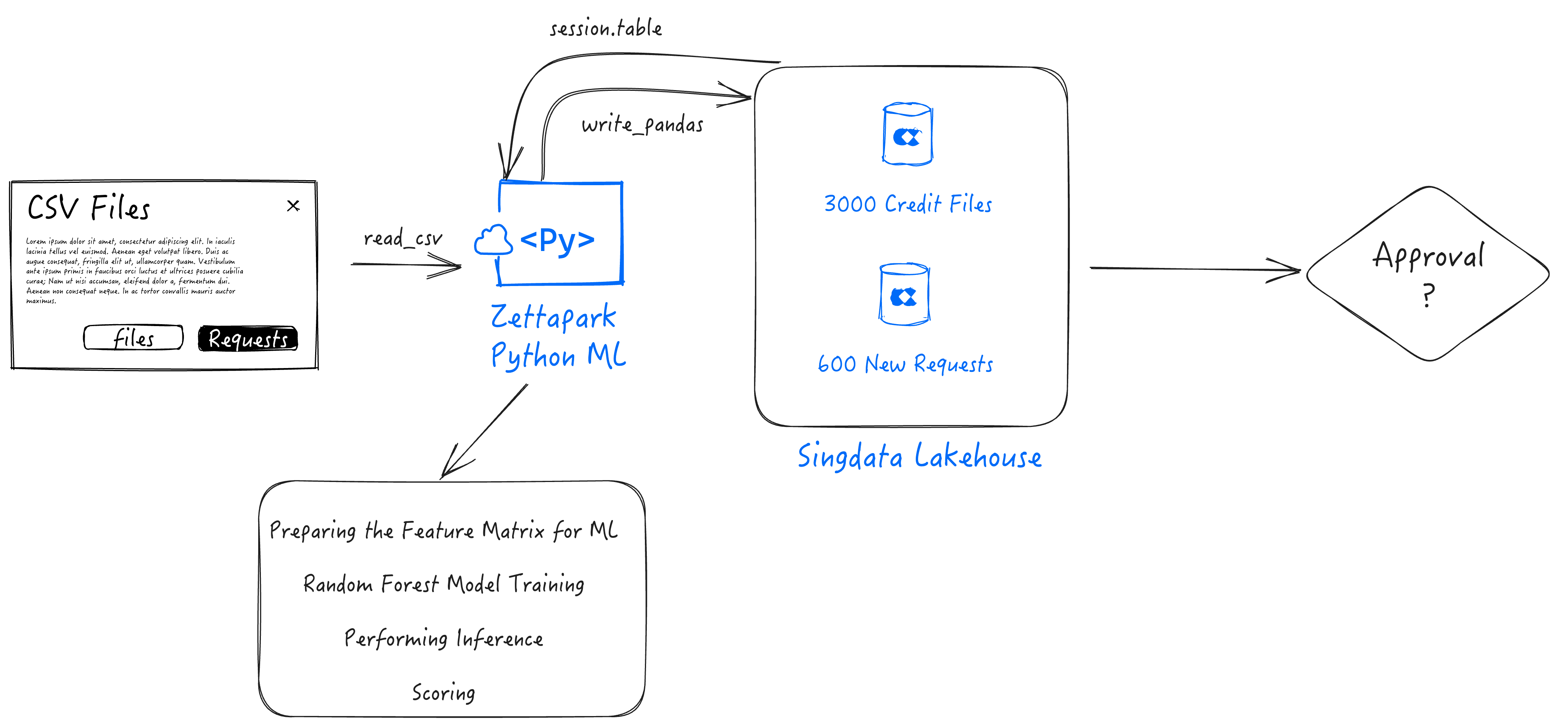
In this notebook, we are going to use the Zettapark Python API to run through a credit card scoring demo.
In this scenario, Zettabank wants to use their existing credit files to analyze the current credit standings on whether the loans are being paid without any issues, and/or if there are any delays/default.
Based on the current credit standing, Zettabank wants to build a machine learning credit scoring algorithm based on the dataset to be able to automate an assessment on whether a loan should be approved or declined.
Prerequisite
Please run the Credit Scoring Demo Setup Notebook prior to running this demo.
1. Data Exploration
In this section, we will explore the dataset for the existing credits.
1.1 Opening a Singdata Lakehouse Session
import json

import pandas as pd
from clickzetta.zettapark import *
from clickzetta.zettapark.functions import *
# read connection para from config file
with open('config/config.json', 'r') as config_file:
    config = json.load(config_file)

schema = config['schema']
vcluster = config['vcluster']

print("Connecting to Lakehouse.....\n")

# create session
session = Session.builder.configs(config).create()

session.sql(f"CREATE SCHEMA IF NOT EXISTS {schema}").collect()
session.sql(f"CREATE VCLUSTER IF NOT EXISTS {vcluster} VCLUSTER_SIZE=1 VCLUSTER_TYPE = GENERAL").collect()

print(session.sql("SELECT current_instance_id(), current_workspace(),current_workspace_id(), current_schema(), current_user(),current_user_id(), current_vcluster()").collect())

print("\nConnected!...\n")
1.2 Explore Data in Lakehouse table
credit_df = session.table("CREDIT_FILES")
credit_df.describe().toPandas()
credit_df.toPandas().info()
<class 'pandas.core.frame.DataFrame'>
RangeIndex: 2940 entries, 0 to 2939
Data columns (total 21 columns):
 #   Column                  Non-Null Count  Dtype
---  ------                  --------------  -----
 0   credit_request_id       2940 non-null   int64
 1   credit_amount           2940 non-null   int64
 2   credit_duration         2940 non-null   int64
 3   purpose                 2940 non-null   object
 4   installment_commitment  2940 non-null   int64
 5   other_parties           271 non-null    object
 6   credit_standing         2940 non-null   object
 7   credit_score            2940 non-null   int64
 8   checking_balance        2940 non-null   float64
 9   savings_balance         2940 non-null   float64
 10  existing_credits        2940 non-null   int64
 11  assets                  2489 non-null   object
 12  housing                 2940 non-null   object
 13  qualification           2940 non-null   object
 14  job_history             2940 non-null   int64
 15  age                     2940 non-null   int64
 16  sex                     2940 non-null   object
 17  marital_status          2940 non-null   object
 18  num_dependents          2940 non-null   int64
 19  residence_since         2940 non-null   int64
 20  other_payment_plans     2940 non-null   object
dtypes: float64(2), int64(10), object(9)
memory usage: 482.5+ KB
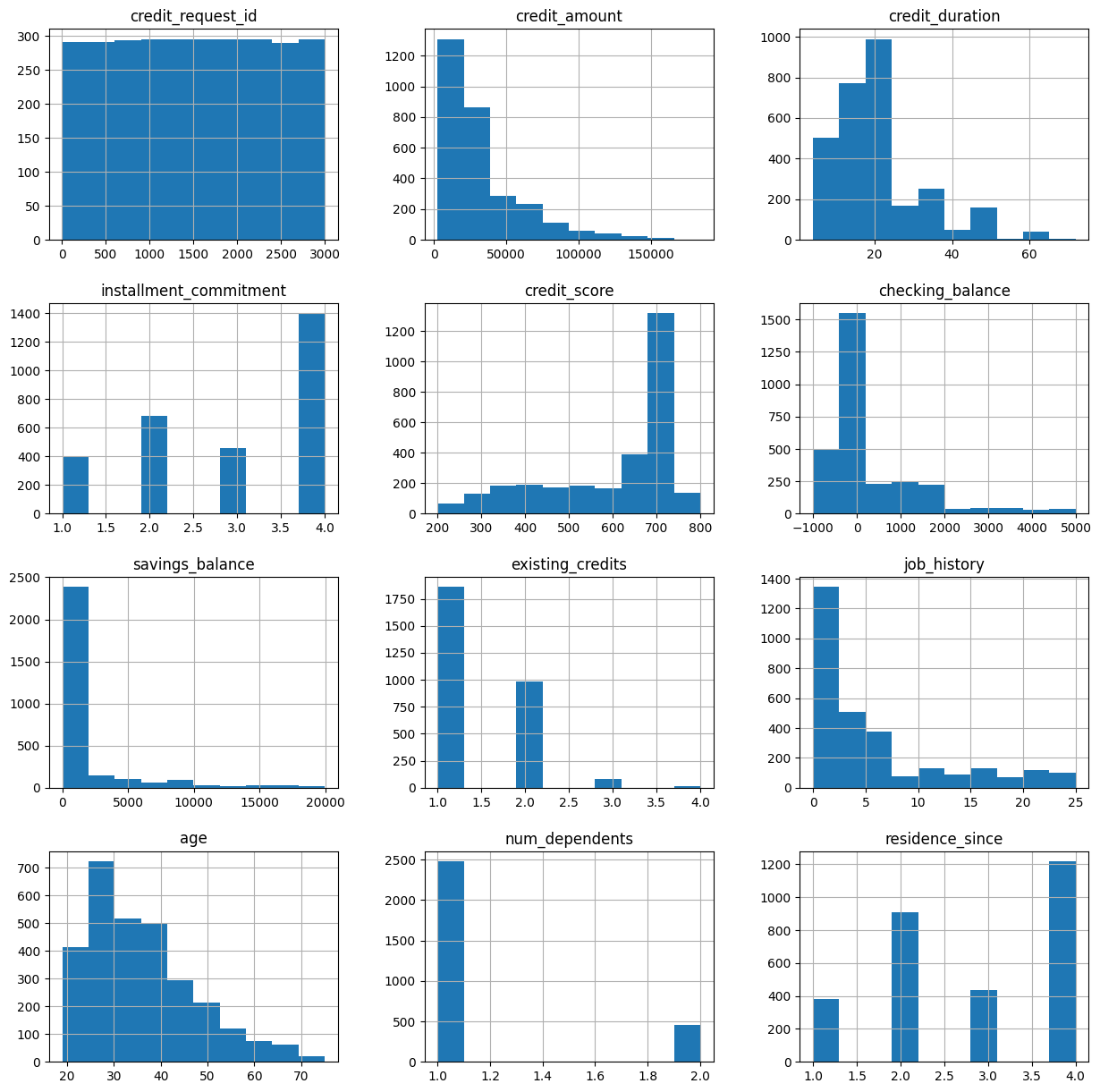
1.3 Visualizing the Numeric Features
From this visualization, we can see a few interesting characteristics:
- Most of the credit requests are for small amounts (< 50k)
- Most of the credit terms are 20 months or less.
- Most of the applicants have a very good credit score.
- Most of the applicants do not have a lot of balance in either credits or savings with Zettabank.
- Most of the applicants are less than 40 years old.
credit_df.toPandas().hist(figsize=(15,15))
array([[<Axes: title={'center': 'credit_request_id'}>,
        <Axes: title={'center': 'credit_amount'}>,
        <Axes: title={'center': 'credit_duration'}>],
       [<Axes: title={'center': 'installment_commitment'}>,
        <Axes: title={'center': 'credit_score'}>,
        <Axes: title={'center': 'checking_balance'}>],
       [<Axes: title={'center': 'savings_balance'}>,
        <Axes: title={'center': 'existing_credits'}>,
        <Axes: title={'center': 'job_history'}>],
       [<Axes: title={'center': 'age'}>,
        <Axes: title={'center': 'num_dependents'}>,
        <Axes: title={'center': 'residence_since'}>]], dtype=object)
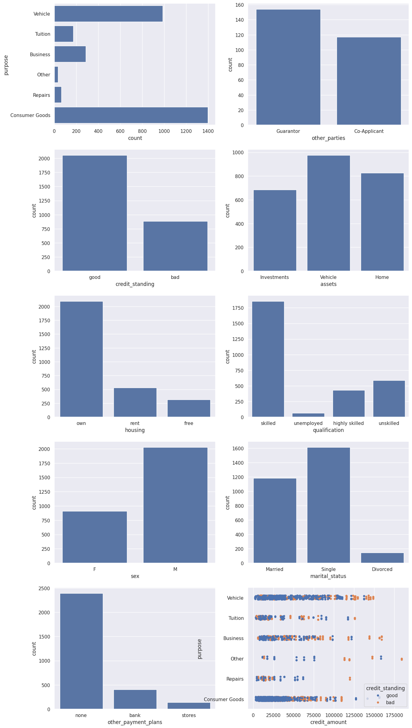
1.4 Visualizing the Categorical Features
From this visualization, we can see a few interesting characteristics:
- Most of the popular credit requests are related to either a vehicle purchase or consumer goods.
- The vast majority of loans do not have guarantors, nor co-applicants.
- Most of credit in file is in good standing.
- The majority of the applicants are male, foreign workers, and skilled who own their own house/apartment.
- Higher amounts of loans (which threshold varies per category of loan) have a higher chance of defaulting.
import matplotlib.pyplot as plt
import seaborn as sns

sns.set(style="darkgrid")

fig, axs = plt.subplots(5, 2, figsize=(15, 30))
df = credit_df.toPandas()
sns.countplot(data=df, y="purpose", ax=axs[0,0])
sns.countplot(data=df, x="other_parties", ax=axs[0,1])
sns.countplot(data=df, x="credit_standing", ax=axs[1,0])
sns.countplot(data=df, x="assets", ax=axs[1,1])
sns.countplot(data=df, x="housing", ax=axs[2,0])
sns.countplot(data=df, x="qualification", ax=axs[2,1])
sns.countplot(data=df, x="sex", ax=axs[3,0])
sns.countplot(data=df, x="marital_status", ax=axs[3,1])
sns.countplot(data=df, x="other_payment_plans", ax=axs[4,0])
sns.stripplot(y="purpose", x="credit_amount", data=df, hue='credit_standing', jitter=True, ax=axs[4,1])
plt.show()
1.5 Running queries through Zettapark API
We can use the Zettapark API to run queries to get various insights. For example, let's try to determine the range of f loans per different category. We can check the Singdata Lakehouse query history and review how the Zettapark API has been pushed down as SQL.
df_loan_status = credit_df.select(col("PURPOSE"),col("CREDIT_AMOUNT"))\
                          .groupBy(col("PURPOSE"))\
                          .agg([min(col("CREDIT_AMOUNT")).as_("MIN_CREDIT_AMOUNT"), max(col("CREDIT_AMOUNT")).as_("MAX_CREDIT_AMOUNT"), median(col("CREDIT_AMOUNT")).as_("MED_CREDIT_AMOUNT"),avg(col("CREDIT_AMOUNT")).as_("AVG_CREDIT_AMOUNT")])\
                          .sort(col("PURPOSE"))
df_loan_status.toPandas()
For the current use case, in order to prepare the data for machine learning, we need to encode the categorical values into numerical.
In order to achieve this, we can leverage Zettapark Python API in order to perform the encoding.
2.1 Preparing the Feature Matrix for ML
In this section, we are going to leverage the Zettapark Python API in order to prepare a feature matrix for a Random Forest Classifier Model.
from clickzetta.zettapark.functions import when

feature_matrix = credit_df.select(
    when(col("purpose") == "Consumer Goods", 1)
    .when(col("purpose") == "Vehicle", 2)
    .when(col("purpose") == "Tuition", 3)
    .when(col("purpose") == "Business", 4)
    .when(col("purpose") == "Repairs", 5)
    .otherwise(0).alias("purpose_code"),
    when(col("qualification") == "unskilled", 1)
    .when(col("qualification") == "skilled", 2)
    .when(col("qualification") == "highly skilled", 3)
    .otherwise(0).alias("qualification_code"),
    when(col("other_parties") == "Guarantor", 1)
    .when(col("other_parties") == "Co-Applicant", 2)
    .otherwise(0).alias("other_parties_code"),
    when(col("other_payment_plans") == "bank", 1)
    .when(col("other_payment_plans") == "stores", 2)
    .otherwise(0).alias("other_payment_plans_code"),
    when(col("housing") == "rent", 1)
    .when(col("housing") == "own", 2)
    .otherwise(0).alias("housing_code"),
    when(col("assets") == "Vehicle", 1)
    .when(col("assets") == "Investments", 2)
    .when(col("assets") == "Home", 3)
    .otherwise(0).alias("assets_code"),
    when(col("sex") == "M", 1)
    .otherwise(0).alias("sex_code"),
    when(col("marital_status") == "Married", 1)
    .when(col("marital_status") == "Single", 2)
    .otherwise(0).alias("marital_status_code"),
    when(col("credit_standing") == "good", 1)
    .otherwise(0).alias("credit_standing_code"),
    col("checking_balance"),
    col("savings_balance"),
    col("age"),
    col("job_history"),
    col("credit_score"),
    col("credit_duration"),
    col("credit_amount"),
    col("residence_since"),
    col("installment_commitment"),
    col("num_dependents"),
    col("existing_credits")
)

feature_matrix_pandas = feature_matrix.toPandas()
print(feature_matrix_pandas)
      purpose_code  qualification_code  other_parties_code  \
0                2                   2                   0
1                2                   2                   0
2                3                   2                   0
3                3                   2                   0
4                2                   2                   0
...            ...                 ...                 ...
2935             0                   0                   0
2936             2                   0                   0
2937             2                   0                   0
2938             2                   2                   0
2939             2                   2                   0

      other_payment_plans_code  housing_code  assets_code  sex_code  \
0                            0             2            0         0
1                            1             1            0         1
2                            0             1            2         0
3                            1             1            2         0
4                            0             2            2         0
...                        ...           ...          ...       ...
2935                         1             0            0         1
2936                         1             0            0         1
2937                         0             0            1         1
2938                         0             2            1         1
2939                         0             2            1         1

      marital_status_code  credit_standing_code  checking_balance  \
0                       1                     1           -728.12
1                       2                     1              0.00
2                       1                     1           4696.00
3                       1                     1            -25.35
4                       1                     1              0.00
...                   ...                   ...               ...
2935                    2                     1           1505.00
2936                    2                     1           4486.00
2937                    2                     1            720.00
2938                    2                     1            752.00
2939                    2                     1           1564.00

      savings_balance  age  job_history  credit_score  credit_duration  \
0               17.00   39           15           466                6
1             2443.00   35            1           202                6
2              143.00   23            1           736               15
3                0.00   23            3           732               12
4              510.00   30            1           507               18
...               ...  ...          ...           ...              ...
2935             0.00   40            0           726               48
2936          7361.86   66            0           343               12
2937           460.00   68            0           396               16
2938          1444.00   27            0           523               45
2939          1998.00   27            0           552               45

      credit_amount  residence_since  installment_commitment  num_dependents  \
0              8600                4                       1               1
1             12040                1                       4               1
2              3920                4                       4               1
3             12000                4                       4               1
4             10550                1                       4               1
...             ...              ...                     ...             ...
2935          53810                4                       3               1
2936          14800                4                       2               1
2937          11750                3                       2               1
2938          45760                4                       3               1
2939          45760                4                       3               1

      existing_credits
0                    2
1                    1
2                    1
3                    1
4                    2
...                ...
2935                 1
2936                 3
2937                 3
2938                 1
2939                 1

[2940 rows x 20 columns]
Now that the feature matrix has been defined, we will convert it into a Pandas Dataframe.
df = feature_matrix.toPandas().astype(int)
<class 'pandas.core.frame.DataFrame'>
RangeIndex: 2940 entries, 0 to 2939
Data columns (total 20 columns):
 #   Column                    Non-Null Count  Dtype
---  ------                    --------------  -----
 0   purpose_code              2940 non-null   int64
 1   qualification_code        2940 non-null   int64
 2   other_parties_code        2940 non-null   int64
 3   other_payment_plans_code  2940 non-null   int64
 4   housing_code              2940 non-null   int64
 5   assets_code               2940 non-null   int64
 6   sex_code                  2940 non-null   int64
 7   marital_status_code       2940 non-null   int64
 8   credit_standing_code      2940 non-null   int64
 9   checking_balance          2940 non-null   int64
 10  savings_balance           2940 non-null   int64
 11  age                       2940 non-null   int64
 12  job_history               2940 non-null   int64
 13  credit_score              2940 non-null   int64
 14  credit_duration           2940 non-null   int64
 15  credit_amount             2940 non-null   int64
 16  residence_since           2940 non-null   int64
 17  installment_commitment    2940 non-null   int64
 18  num_dependents            2940 non-null   int64
 19  existing_credits          2940 non-null   int64
dtypes: int64(20)
memory usage: 459.5 KB
This is what the data looks like:
3. Random Forest Model Training
We are going to leverage the Random Forest Classifier Model available as part of the scikit-learn popular ML Library available in Python.
from sklearn.model_selection import train_test_split

X_train, X_test, y_train, y_test = train_test_split(df.drop('credit_standing_code', axis=1),
                                                    df['credit_standing_code'], test_size=0.30)
from sklearn.ensemble import RandomForestClassifier

rfc = RandomForestClassifier(n_estimators=100)
rfc.fit(X_train, y_train)
4. Testing the Model
rfc_pred = rfc.predict(X_test)
from sklearn.metrics import classification_report, confusion_matrix

print(classification_report(y_test,rfc_pred))
              precision    recall  f1-score   support

           0       0.99      0.87      0.92       275
           1       0.94      1.00      0.97       607

    accuracy                           0.96       882
   macro avg       0.97      0.93      0.95       882
weighted avg       0.96      0.96      0.95       882
print(confusion_matrix(y_test,rfc_pred))
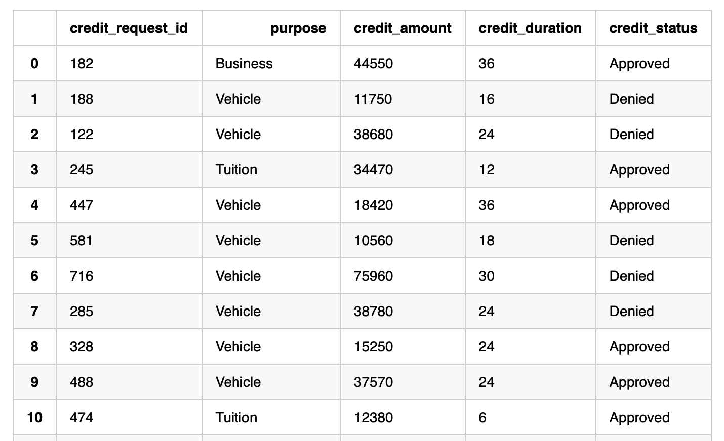
In the example below, we want to process an existing batch of 60 credit pending requests and provide an assessment on whether the loan should be approved or denied. The data looks like as follows:
df_cred_req = session.table("CREDIT_REQUESTS")
<class 'pandas.core.frame.DataFrame'>
RangeIndex: 2940 entries, 0 to 2939
Data columns (total 20 columns):
 #   Column                    Non-Null Count  Dtype
---  ------                    --------------  -----
 0   purpose_code              2940 non-null   int64
 1   qualification_code        2940 non-null   int64
 2   other_parties_code        2940 non-null   int64
 3   other_payment_plans_code  2940 non-null   int64
 4   housing_code              2940 non-null   int64
 5   assets_code               2940 non-null   int64
 6   sex_code                  2940 non-null   int64
 7   marital_status_code       2940 non-null   int64
 8   credit_standing_code      2940 non-null   int64
 9   checking_balance          2940 non-null   int64
 10  savings_balance           2940 non-null   int64
 11  age                       2940 non-null   int64
 12  job_history               2940 non-null   int64
 13  credit_score              2940 non-null   int64
 14  credit_duration           2940 non-null   int64
 15  credit_amount             2940 non-null   int64
 16  residence_since           2940 non-null   int64
 17  installment_commitment    2940 non-null   int64
 18  num_dependents            2940 non-null   int64
 19  existing_credits          2940 non-null   int64
dtypes: int64(20)
memory usage: 459.5 KB
6. Develop Function for scoring
As the Zettabank receives the credit requests in near real-time, we want to write a Function which could be called through a task to score micro-batches of requests as they come in.
The Python Function will first build the input features for the model using the Zettapark API for scoring.
from clickzetta.zettapark.functions import col, when

def process_credit_requests_fn (session, credit_requests: str, credit_assessment: str) -> int:

    #Build the input features for the model using the Zettapark API with direct encoding.
    df_cred_req = session.table(credit_requests).select(
                            col("CREDIT_REQUEST_ID"), col("PURPOSE"),
                            when(col("PURPOSE") == "Consumer Goods", 1)
                            .when(col("PURPOSE") == "Vehicle", 2)
                            .when(col("PURPOSE") == "Tuition", 3)
                            .when(col("PURPOSE") == "Business", 4)
                            .when(col("PURPOSE") == "Repairs", 5)
                            .otherwise(0).alias("PURPOSE_CODE"),
                            when(col("QUALIFICATION") == "unskilled", 1)
                            .when(col("QUALIFICATION") == "skilled", 2)
                            .when(col("QUALIFICATION") == "highly skilled", 3)
                            .otherwise(0).alias("QUALIFICATION_CODE"),
                            when(col("OTHER_PARTIES") == "Guarantor", 1)
                            .when(col("OTHER_PARTIES") == "Co-Applicant", 2)
                            .otherwise(0).alias("OTHER_PARTIES_CODE"),
                            when(col("OTHER_PAYMENT_PLANS") == "bank", 1)
                            .when(col("OTHER_PAYMENT_PLANS") == "stores", 2)
                            .otherwise(0).alias("OTHER_PAYMENT_PLANS_CODE"),
                            when(col("HOUSING") == "rent", 1)
                            .when(col("HOUSING") == "own", 2)
                            .otherwise(0).alias("HOUSING_CODE"),
                            when(col("ASSETS") == "Vehicle", 1)
                            .when(col("ASSETS") == "Investments", 2)
                            .when(col("ASSETS") == "Home", 3)
                            .otherwise(0).alias("ASSETS_CODE"),
                            when(col("SEX") == "M", 1)
                            .otherwise(0).alias("SEX_CODE"),
                            when(col("MARITAL_STATUS") == "Married", 1)
                            .when(col("MARITAL_STATUS") == "Single", 2)
                            .otherwise(0).alias("MARITAL_STATUS_CODE"),
                            col("CHECKING_BALANCE"),
                            col("SAVINGS_BALANCE"),
                            col("AGE"),
                            col("JOB_HISTORY"),
                            col("CREDIT_SCORE"),
                            col("CREDIT_DURATION"),
                            col("CREDIT_AMOUNT"),
                            col("RESIDENCE_SINCE"),
                            col("INSTALLMENT_COMMITMENT"),
                            col("NUM_DEPENDENTS"),
                            col("EXISTING_CREDITS")
                         )

    # Call the UDF to score the existing credit requests read previously
    input_features = [ 'PURPOSE_CODE',
                   'QUALIFICATION_CODE',
                   'OTHER_PARTIES_CODE',
                   'OTHER_PAYMENT_PLANS_CODE',
                   'HOUSING_CODE',
                   'ASSETS_CODE',
                   'SEX_CODE',
                   'MARITAL_STATUS_CODE',
                   'CHECKING_BALANCE',
                   'SAVINGS_BALANCE',
                   'AGE',
                   'JOB_HISTORY',
                   'CREDIT_SCORE',
                   'CREDIT_DURATION',
                   'CREDIT_AMOUNT',
                   'RESIDENCE_SINCE',
                   'INSTALLMENT_COMMITMENT',
                   'NUM_DEPENDENTS',
                   'EXISTING_CREDITS']

    df_assessment = df_cred_req.select(
                    col("CREDIT_REQUEST_ID"), col("PURPOSE"), col("CREDIT_AMOUNT"), col("CREDIT_DURATION"),
                    when(col("CREDIT_SCORE") > 600, "Approved").otherwise("Denied").alias("CREDIT_STATUS"))

    df_assessment.write.mode("overwrite").saveAsTable(credit_assessment)

    #The function will return the total number of credit requests assessed.
    return df_assessment.count()
7. Invoking the Function for scoring
process_credit_requests_fn (session, "credit_requests", "credit_assessments")
session.table("credit_assessments").toPandas()
Appendix: