Learn Product Function Usage Based on BI Analysis Scenarios

This chapter will help you quickly get started with the core functional modules of Singdata Lakehouse Studio through real business scenario cases, and guide you to complete the end-to-end workflow from business databases to data applications. Through the introduction of this chapter, you will learn:

How to configure data sources
How to create data integration tasks
How to create data development tasks
How to configure and publish task scheduling
How to perform task instance operations and maintenance
How to connect to BI tools via JDBC
How to create and call UDF functions

Scenario Introduction

Enterprise business intelligence (BI) generally obtains raw data from the enterprise's business systems, with the backend databases of business systems typically being relational databases such as MySQL, Oracle, etc. This scenario uses a MySQL database as an example to complete ① data source configuration, ② data integration, ③ data development, ④ task scheduling configuration and publishing, ⑤ task instance operations and maintenance, and ⑥ connecting to BI tools via JDBC to meet BI data analysis business requirements through Singdata Studio.

Workflow Diagram

Business Requirements

The business requirements in this example simulate common BI analysis scenarios in e-commerce, generating a wide table at the detailed layer of the data warehouse by associating user behavior log data with dimension tables such as products, stores, and time zones. This wide table is then provided to downstream data application layers, and BI tools are used for sales and order statistics, funnel conversion models, popular product displays, etc.

The overall workflow construction idea is:

Complete the creation of data integration tasks for these 4 tables

Create 4 Lakehouse target tables, 1 business real-time table, and 3 dimension tables

Create data development tasks

Use SQL join queries to merge the fields of the four tables into a wide table and write it into a DWD layer result table

Configure task dependencies in the order of data integration tasks first, followed by SQL tasks

Deploy all tasks to the production environment.

Review Preparations

Refer to the Preparations in the previous chapter. Before starting the "Quick Start," you need to ensure that your enterprise has activated the Singdata Lakehouse service and can log in to the Studio product homepage.

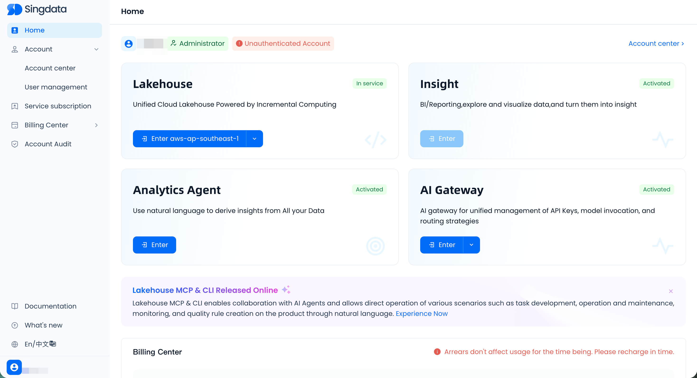
In the initialized product environment, you may already have the following object resources:

Default user (User): Your Username —— Figure 1
Default workspace: quickstart_ws —— Figure 2
Default Schema: public —— Figure 3
Default computing clusters: General-purpose cluster: DEFAULT, Analytical cluster: DEFAULT_AP —— Figure 4

Figure 1 —— User

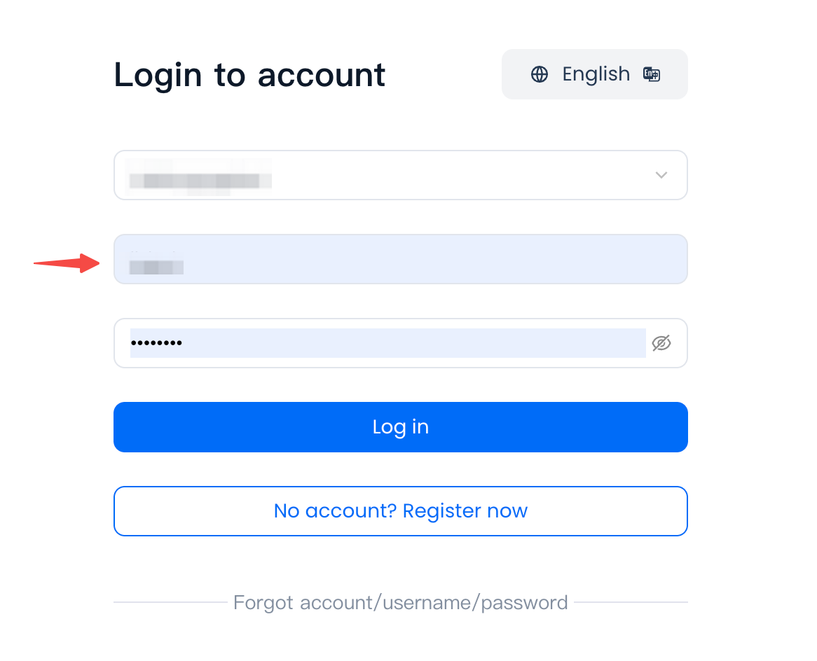
Figure 2 —— Workspace: QuickStart_WorkSpace

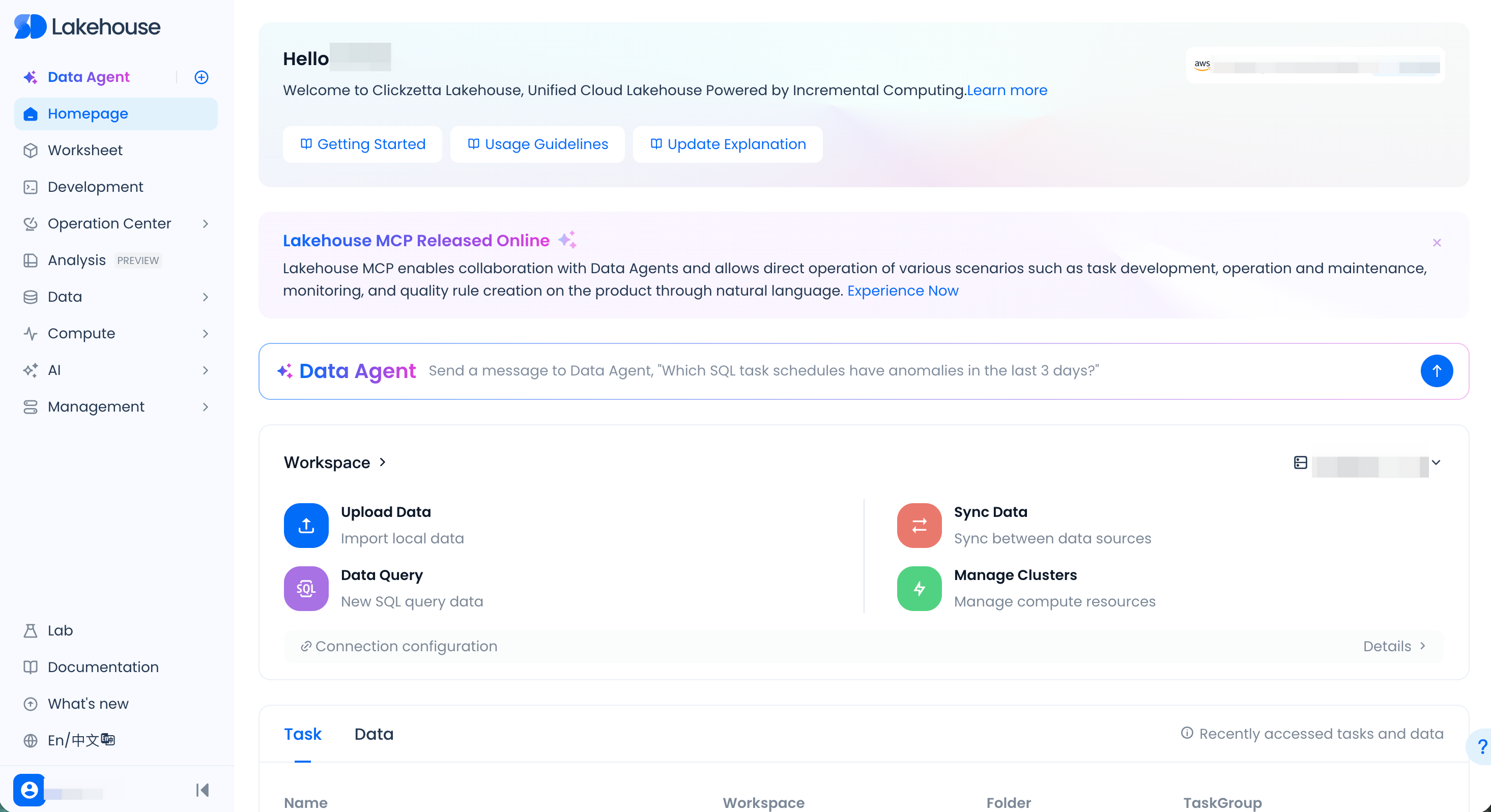
Figure 3 —— Schema: Public

Figure 4 —— Computing Cluster: Default

Start Working

Next, we will proceed step by step, starting with connecting to the business system's database.

[Configure Data Source]

Studio provides two ways to create a new data source:

Method 1: Follow the steps ① [Manage] → ② [Data Source] → ③ [New Data Source] to create a new data source;
Method 2: Follow the steps ① [Develop] → ② ["✙" button] → ③ [Offline Sync] → ④ ["✙" button] to create a new data source.

Figure 1 —— Method 1

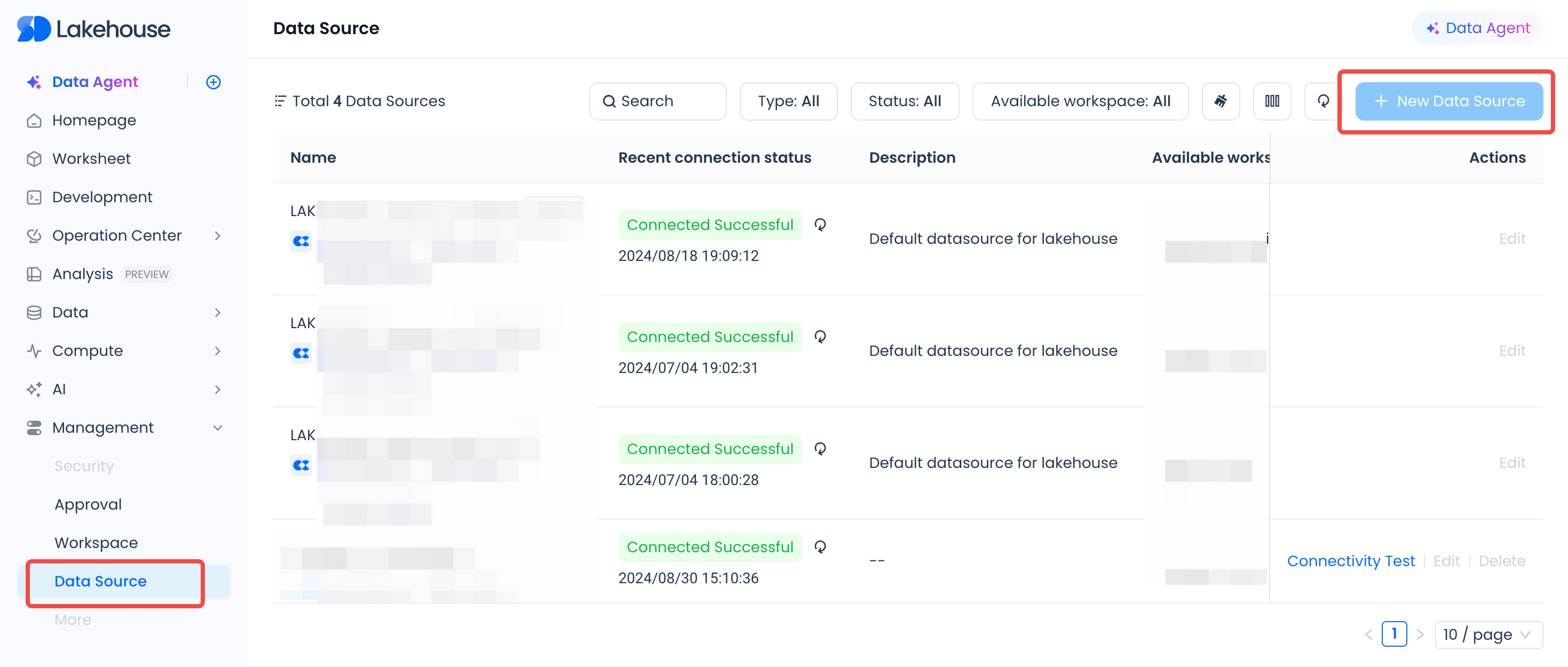
Figure 2 —— Method 2

Select the MySQL type data source on the new data source page and click Next.

Enter the database connection information and click connectivity test. If the configuration is correct, a green [Connection Successful] will be displayed. If the connection test fails, you need to verify the configuration information or change the database's access whitelist policy. *If you need to add specific IP whitelist entries, please contact Singdata customer service or your account manager.

After successful creation, the data source can be seen in the list.

【Create Data Integration Task】

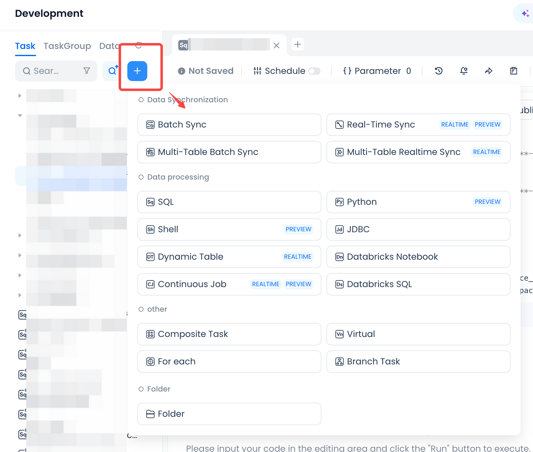
Let us go back to the [Development] menu and create an [Offline Synchronization Task]

Temporarily name the task “MYSQL Data Integration Task” here and click OK.

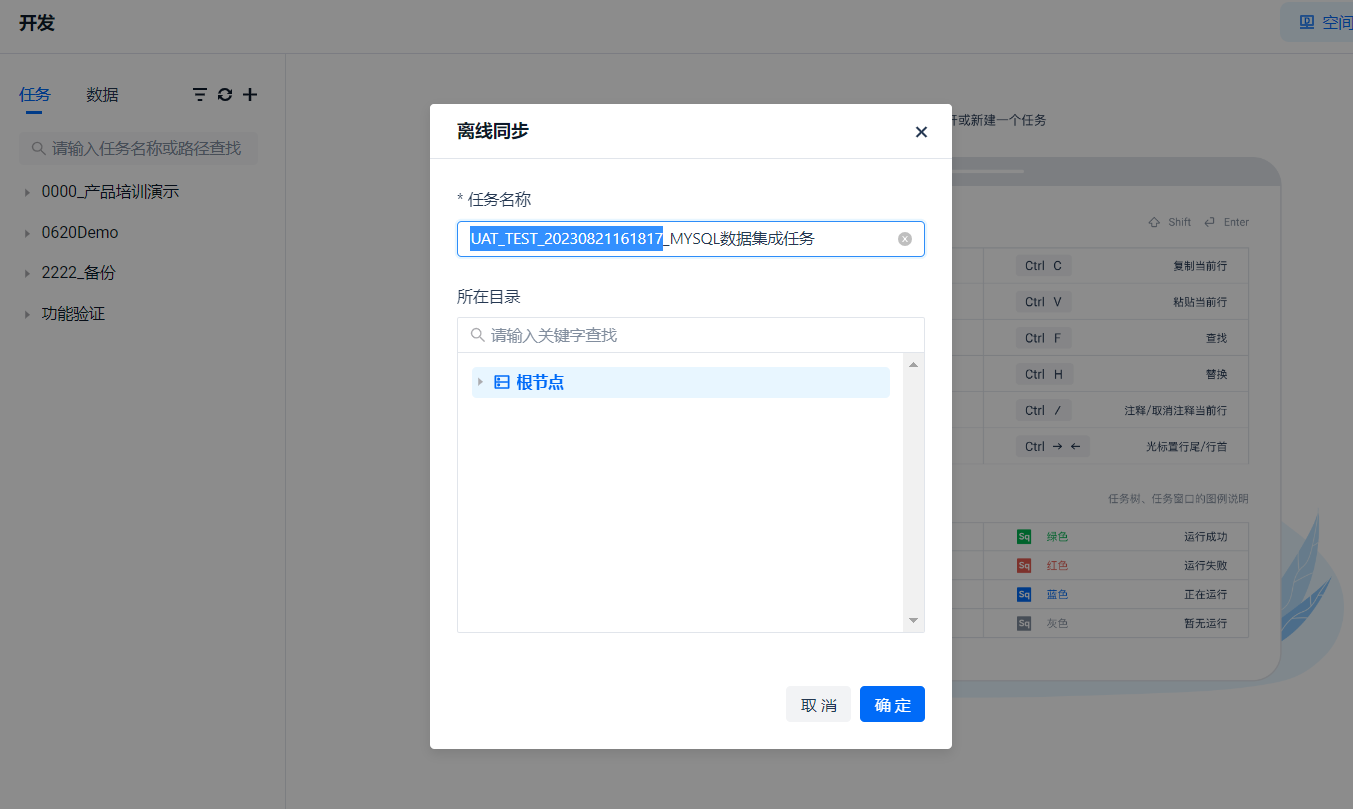
You can see the task you just created at ① in the list. Click ② to select the data source type as MYSQL at ③, and select the data source name we just created: BizData_Demo

Select the database at ①, select the table at ②, add filter conditions at ③, and click the button at ④ to preview the data. splitPk is a split key for multi-concurrent data extraction. It splits data based on the INT type primary key of the table in the database. It is not required and will not be demonstrated in depth here.

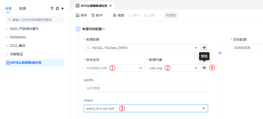
After clicking the [Preview] button, a small amount of data will be previewed based on the configured filter conditions.

Since we are synchronizing data from the MySQL data source to Singdata Lakehouse, the target data source is naturally the Lakehouse type, as shown in steps ① → ② → ③ below

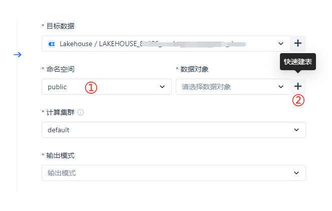
The namespace at ① can first select the default public. Since this is the first time creating a task and the table has not been created on the Lakehouse side, the data object at ② provides a convenient one-click table creation feature.

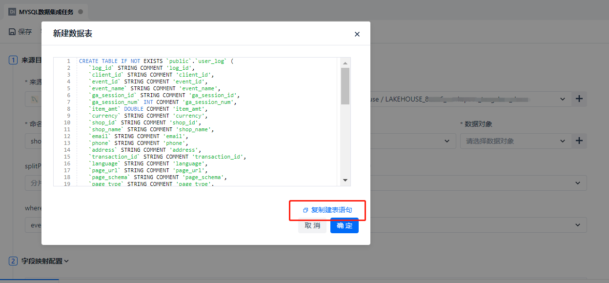
In the pop-up one-click table creation window, clicking the [Confirm] button will directly create the Lakehouse table. In addition, it also supports copying the table creation statement, making it convenient for users to modify and then perform the creation operation separately.

Note: The DDL statement for one-click table creation does not create a [Partitioned Table] and does not include partition fields. If you want to create a partitioned table in Lakehouse, please modify the DDL statement for table creation. For the partition table creation syntax, refer to the [SQL Reference] chapter.

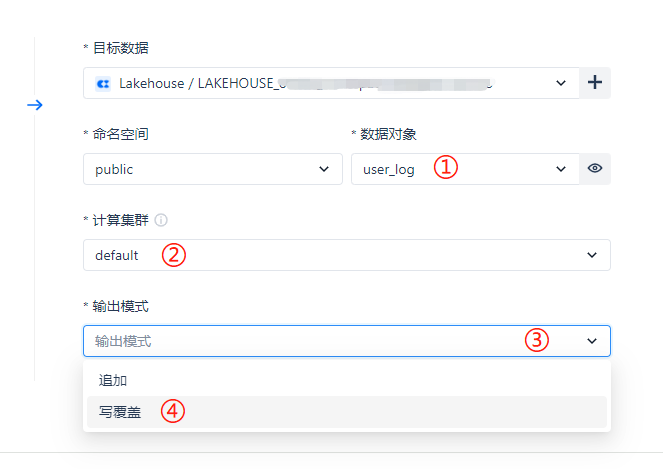
After creating the target table, the table will be directly selected in the data object at ①. The computing cluster at ② does not need to be changed, and the default cluster is selected by default. For the output mode selection at ③, since we are doing full data synchronization, the [Write Overwrite] mode at ④ is generally selected.

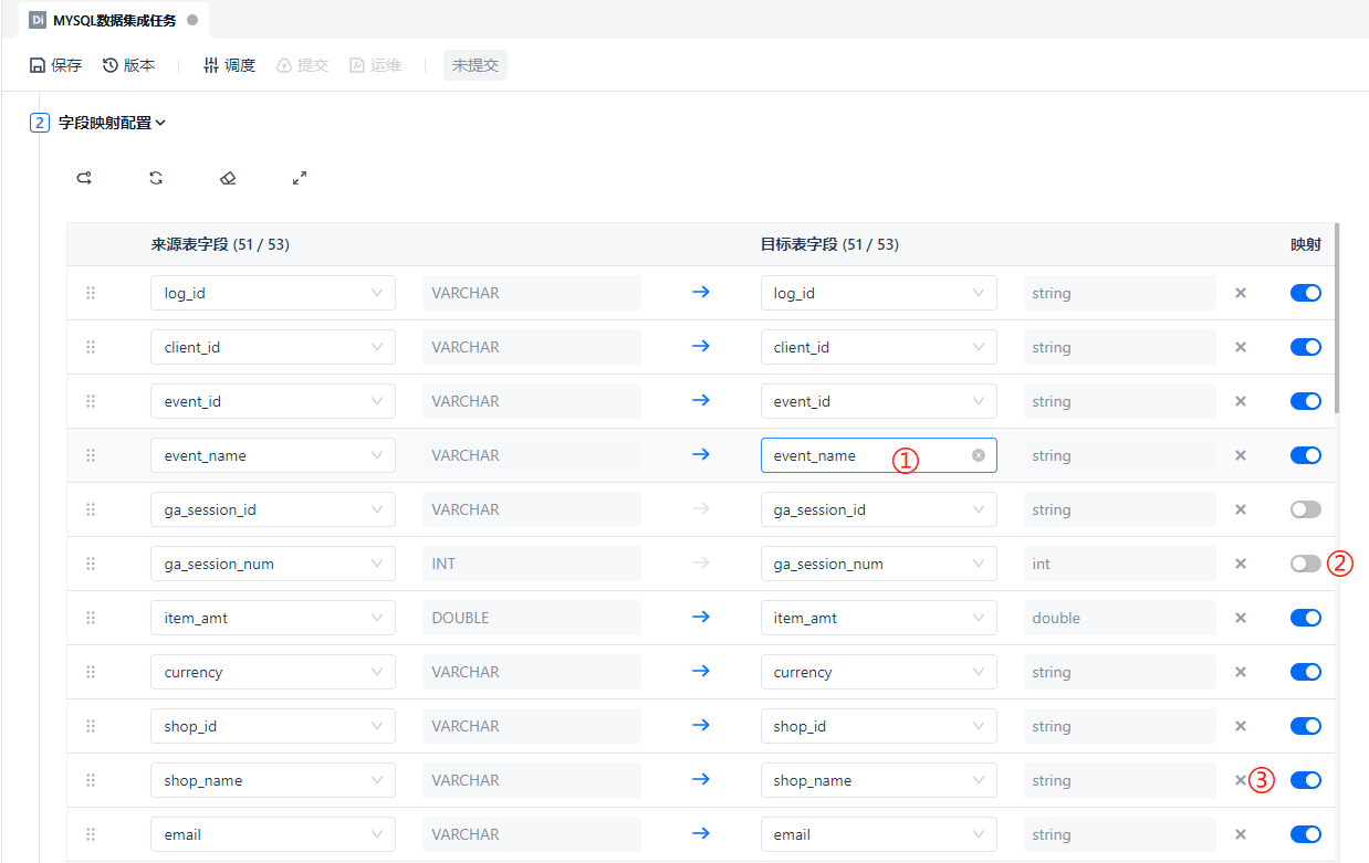
After selecting the source table and target table, the field mapping configuration below will be displayed. Position ① supports directly modifying the target field name, position ② supports enabling the field mapping for that row or temporarily disabling it (other fields are not affected), and position ③ supports deleting a single row's field mapping to reduce some clearly unnecessary fields.

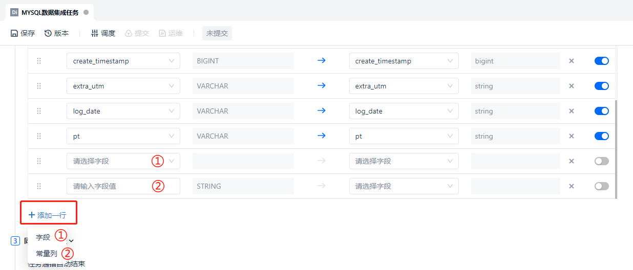
At the bottom of the field mapping, manual field addition or constant columns are also supported. Manually added fields can repeatedly obtain the value of a field from the source table and assign it to another field in the target. Constant columns support lightweight processing and transformation during data synchronization, allowing fixed values or function expressions to be assigned to target fields. This operation is not involved in this example, so it will not be demonstrated.

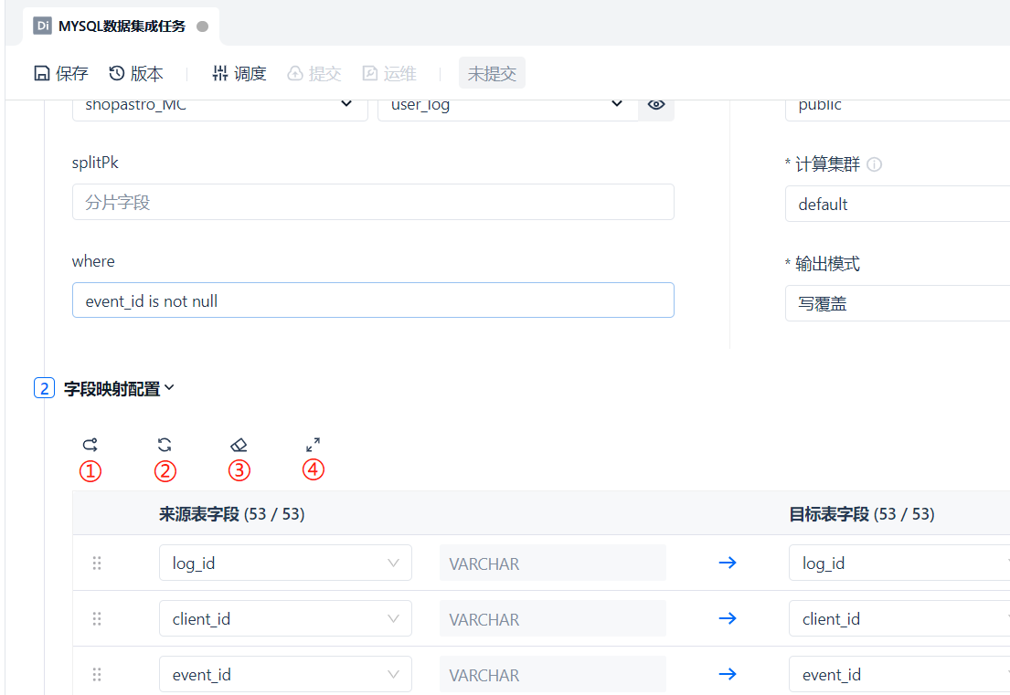
So what if the field mapping is filled in incorrectly and you want to reset the field mapping relationship? Here we have also thoughtfully prepared reset and refresh functions, which are ① Same-Name Mapping, ② Reset and Refresh, ③ Clear Mapping, and ④ Full Screen.

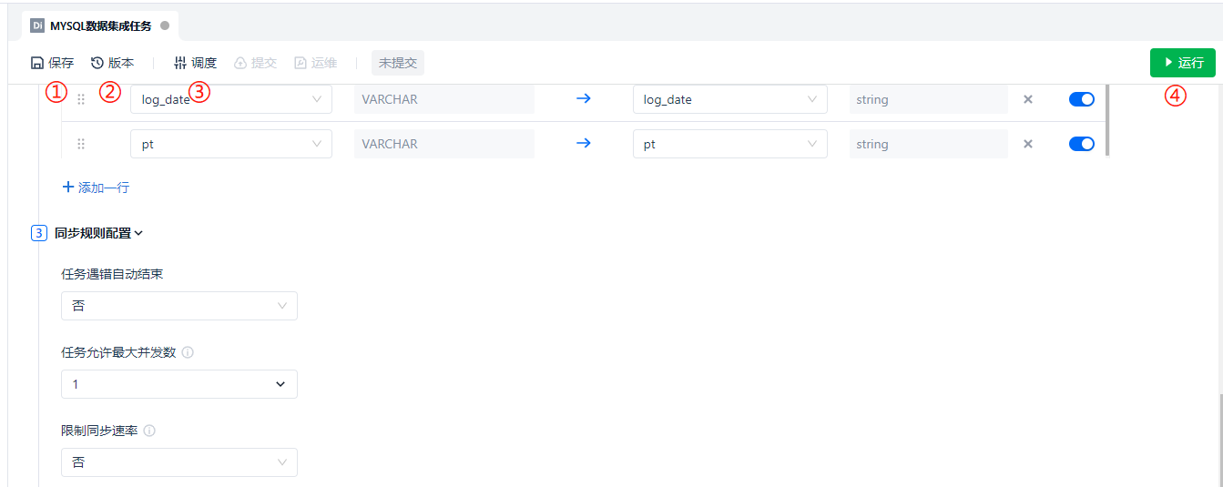
After the task configuration is completed, the [Save] button located at ① can be used to save the task, and the [Version] button located at ② can be used to view historical version information, which will not be elaborated here. It is worth mentioning that after the [Schedule] configuration located at ③ is completed, the [Submit] button will be unlocked. Only when the task is submitted to the production environment will the job be scheduled according to the scheduling configuration. Therefore, after the task is [Submitted], the [Operations] button will be unlocked.

However, after saving the task, we usually click the [Run] button located at ④ to try to run the task manually and complete the initial data integration.

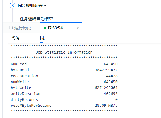
After clicking [Run] to start the task, the [Run] button at ① will become the [Stop] button, and a new entry will be added to the running history below. The task instance that is running is marked at ②, and the task running details can generally be viewed by checking the [Log] at ③ in the operation column on the right.

The log information is shown as follows:

Next, just wait for the task to complete. At this point, the data has been written into the Singdata Lakehouse.

【Configure Scheduling Dependencies】

Let's not rush to check the data count, but continue to complete the scheduling configuration. Click the [Schedule] button in the top function menu, and the scheduling menu will slide out from the right. We fast forward to the [Scheduling Time] section: in the offline T+1 scenario, the scheduling cycle is configured as [Daily Scheduling], [Execute Once], [Start Scheduling at 00:00], effective on the same day, and [Never Expires].

Among them, ① can also be selected as [Specified Days of the Month] or [Specified Days of the Week], and ② can be selected as [Execute Multiple Times] with an interval of X minutes for the scheduling cycle.

In the [Instance Information] section, since we have just run the task, the instance generation method at ③ can be selected as [Effective the Next Day]. (Note: For tasks that run multiple times a day, choose [Effective After Release] after publishing, otherwise, it will start running the next day)

[Retry on Error] is the strategy for handling task error retries. Usually, we choose [Retry Regardless of Success or Failure], which will not be elaborated here.

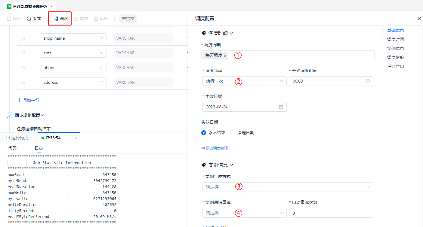
Finally, we come to ① [Scheduling Dependencies] and ② [Task Output]. After completing the configuration, click the ③ [Confirm] button to unlock the [Submit] button, which means the task is ready to be submitted to the production environment for job scheduling.

Regarding [Scheduling Dependencies], we all know that a standard data warehouse processing process starts with data integration, so data integration tasks are usually the starting node of the entire chain and have no upstream dependent tasks. Therefore, no settings are made for [Scheduling Dependencies] at ①. Of course, data integration tasks generally do not take a whole day, so there is no need to check [Self-Dependency] below.

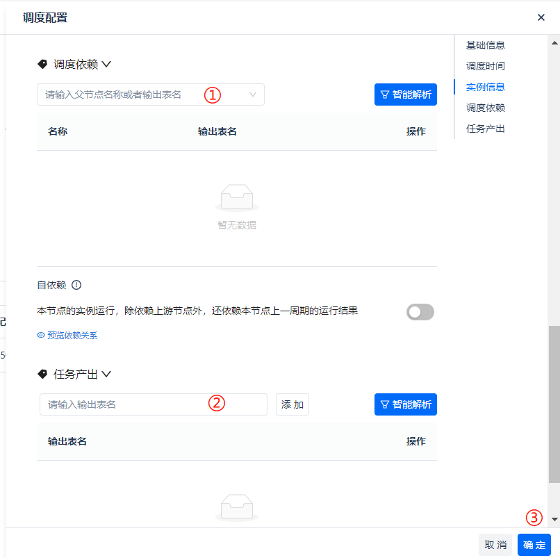
Regarding [Task Output], first, we need to explain what task output is for: the purpose of the currently configured data integration task is to write the data of the corresponding table from the source database into the target table at the destination. Therefore, in the entire scheduling system, it is necessary to declare that this target table is "produced" by this task, i.e., "task output."

The table name defined here for task output must not only be the "physical real name" of the target table but can also be other "aliases" manually changed, or even multiple different aliases. Its main function is to allow the table produced by this task to be searchable by other tasks in the entire scheduling dependency system, thereby forming upstream and downstream dependencies. Its greatest application is to be relied upon by other tasks in the scheduling system.

Therefore, this section provides buttons for manually adding table names and the system's [Intelligent Parsing] function. In this example, no special adjustments are made to aliases, so we directly choose [Intelligent Parsing], as shown in the figure.

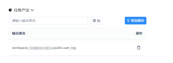
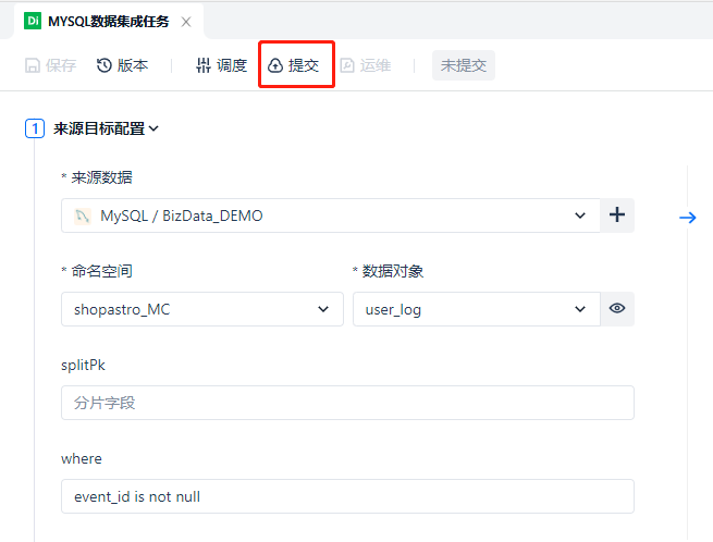
After completing the configuration, click [Confirm] to unlock the [Submit] button.

【Submit and Publish Task】

Click the [Submit] button, and a confirmation window comparing with historical versions will pop up. In this example, it is the first submission, so just click [Confirm].

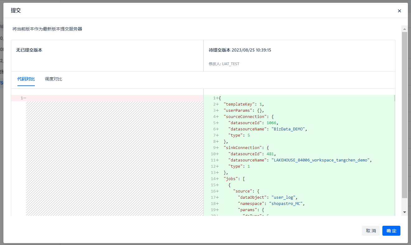
After the submission is successful, a prompt will pop up, and the task status will change from [Not Submitted] to [Submitted].

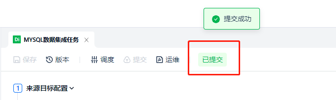
At this point, a data integration task has been successfully published. Next, we may have two questions:

Just synchronized the data, should I check the data volume and preview it?
The data integration task has been published to the scheduling system, how do I operate and view these tasks?

We will explain the above two issues in the following chapters: [Data Development] and [Task Instance Operation and Maintenance].

[Create Data Development Task]

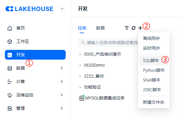
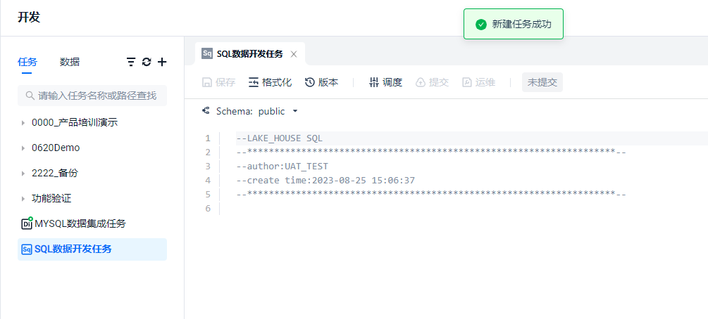
Create an SQL task as shown in the figure, and you can enter the SQL editor page. We will first conduct some basic data exploration, such as checking the data volume of the newly accessed table and previewing some data.

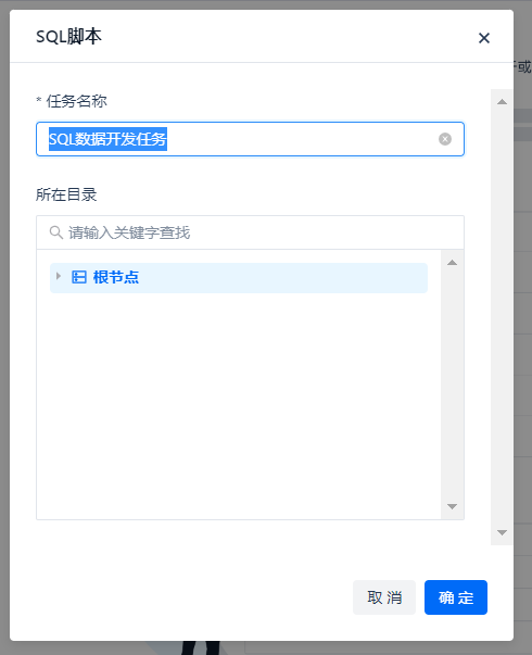
The task name is tentatively set as "SQL Data Development Task", click OK.

After the creation is successful, enter the SQL editor. The function buttons are roughly the same as the data integration task, with an additional [Format] button for beautifying SQL.

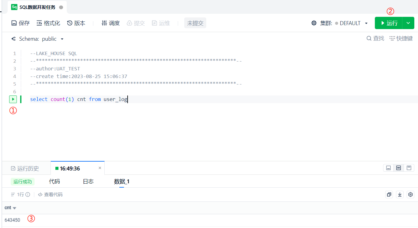
Query the result through the statement of counting table entries. You can execute the query locally/single line at ①, and the entire script will run the task at ②. Regardless of whether you use ① or ②, the results are viewed at ③.

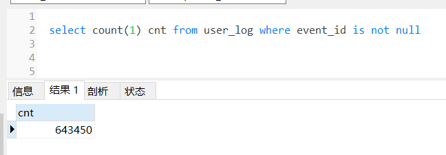
Then we query the number of entries in this table in the source database, and we can find that the number of entries on both sides is consistent. (Don't forget that we added event_id is not null in the [Filter] of data integration, and this condition should also be added when querying the source database)

Okay, the data volume on both sides is consistent. Then use a script similar to the following to preview the data and see if the data format is correct, etc.

Up to this step, the basic data exploration has been completed. Next, we will build the entire workflow.

Let's confirm the business goal again: We have configured the data source from left to right, and learned how to create data integration tasks and data development tasks.

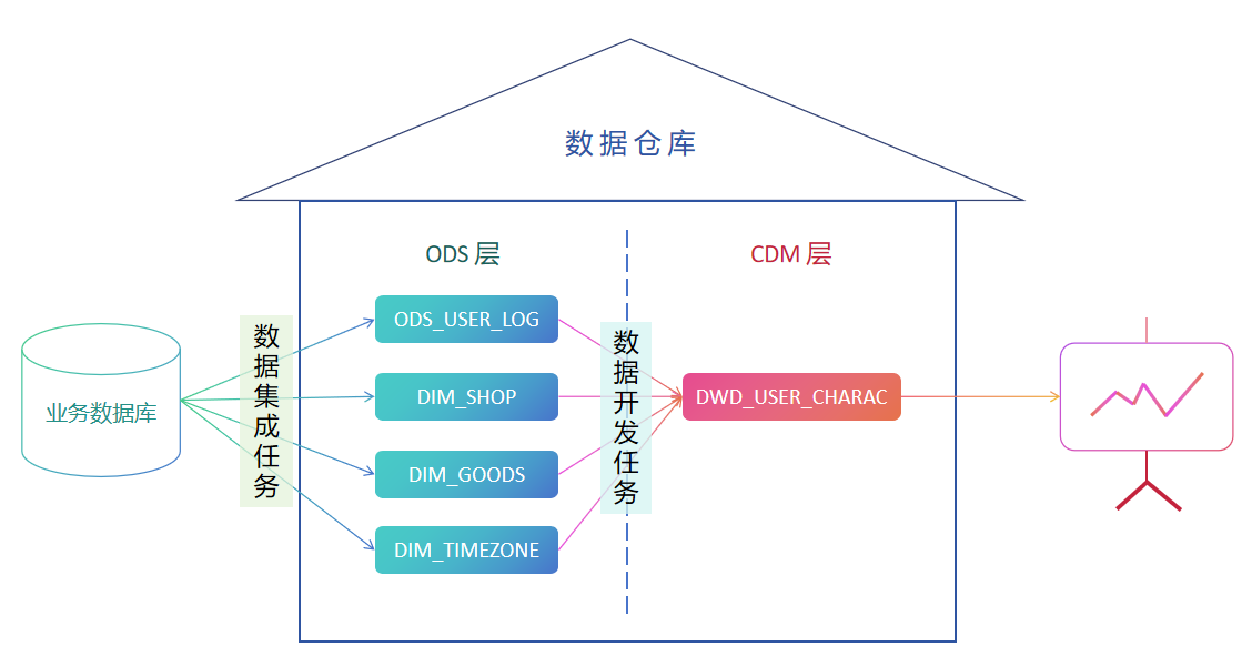
So, we just need to repeat the process of [creating data integration tasks] multiple times to create these 4 tables and import the data into Singdata Lakehouse.

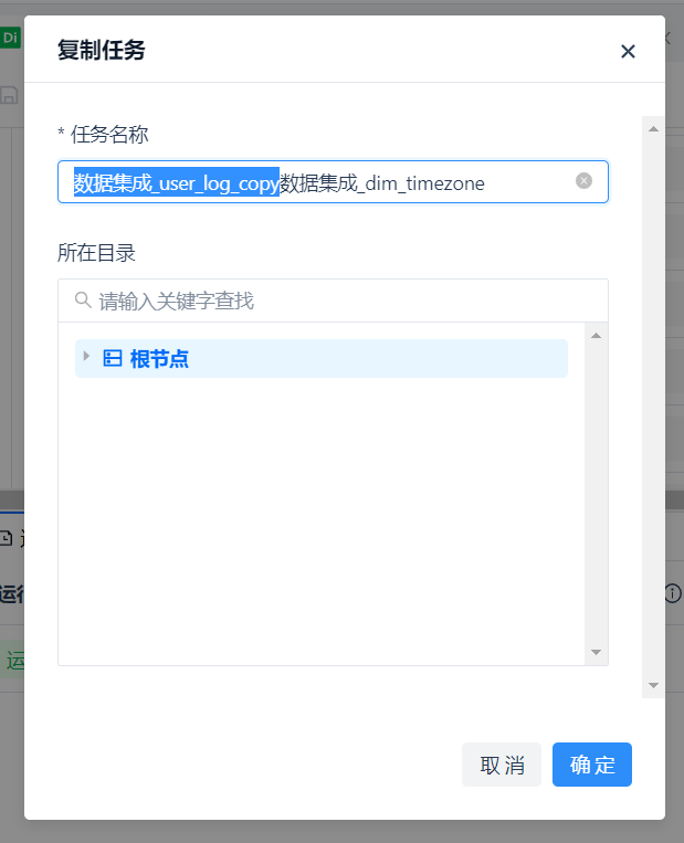
Using the [Copy] function in the [More] options on the right side of the task name, you can quickly copy 4 tasks from the same data source, slightly modify the configuration, and create the target tables with one click, making it very convenient to complete the task creation.

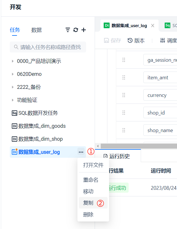
The copied task names will have "_copy" added to the original task name by default. Here, you just need to change it to the desired name as needed.

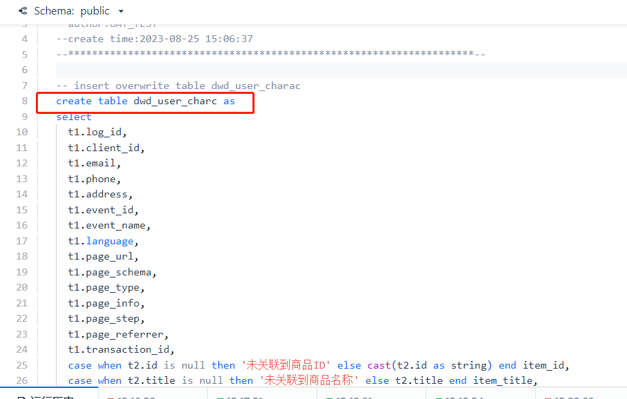
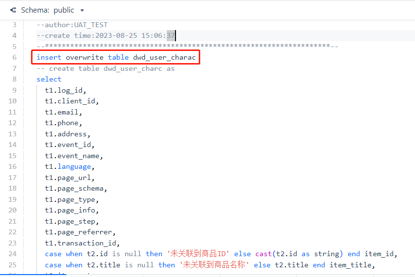
Next, modify the script content in the data development task to complete the join query of the user_log table with the shop, goods, and timezone dimension tables, and write the result into dwd_user_charac. If it is the first time creating the table, you can use the create table xxx as select... statement and run it once separately. Of course, if you need to schedule the task daily, the final submitted task should use [insert overwrite] for writing.

Select the upstream scheduling dependencies through fuzzy search.

We can only execute the SQL processing task after all data integration tasks are completed, so just add the four upstream tasks.

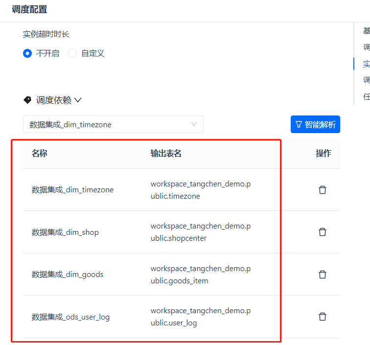
Other configurations are the same as the methods mentioned above. Finally, don't forget to [Save] and [Submit]. All submitted task icons should have a green circle badge.

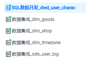
Okay, at this point, we have completed the creation of all data integration tasks and data development tasks, and have run a round of tasks. Next, we will introduce how to view these task instances and lineage relationships in the [Operations Center].

[Task Operations]

After the task is submitted to production, we will introduce some basic operations work. Click [Task Operations] at position ① in the left menu bar to enter the Operations Center. The tabs ②③④⑤ represent [Periodic Tasks], [Real-time Tasks], [Supplementary Tasks], and [Task Instances] respectively.

When we click to enter the [Task Operations] module, the page defaults to the [Task Instances] tab ④, because operations personnel generally care about the daily running status and results of task instances. Task instances are divided into [Periodic Instances] ⑥ and [Temporary Instances] ⑦, with running statuses of [Running Successfully] ⑧, [Running] ⑨, and [Running Failed] ⑩.

Here we need to understand the difference between [Tasks] and [Instances]: A task refers to a preset workflow configuration, while an instance is the instantiation of these workflow configurations, i.e., the actual execution example.

We click the periodic task tab to view our published SQL data development tasks and enter the task details page.

The task details page, in addition to its own information [Task Details] ①, also provides tabs for viewing [Task Instances] ②, [Node Code] ③, and [Operation Logs] ④. Here, only the task details tab is displayed. The upper part of the task details shows some metadata information about the task.

The lower part shows the dependency relationships between the task and its upstream and downstream tasks.

So, the above is the task details. In the instance details, you can also see the running status of the instance. Similar to the task details, the nodes show the actual running status of the instance and support operations such as setting success, setting failure, and rerunning. These will not be elaborated here.

[Connecting BI Tools]

Based on the above content, we assume that all data preparation work has been completed. The next step is the application of the data. In this example, the data processed in the data warehouse is finally displayed on the BI dashboard.

First, we need to understand that Singdata Lakehouse provides a rich SDK that allows BI tools to directly connect and access Lakehouse via JDBC or Python SqlAlchemy. Therefore, most conventional BI tools on the market, such as FanRuan BI, SuperSet, Tableau, Hengshi BI, Power BI, etc., are mostly supported.

Taking FanRuan BI as an example, we can first go to the < JAVA SDK Introduction> section to get the JDBC Driver.

After downloading the JAVA SDK, we need to add this Driver to the third-party data connection driver in the system settings of FanRuan BI. FanRuan BI is a bit special; by default, it does not allow users to upload drivers locally, and you need to enable the switch in the backend. Refer to the official documentation for the steps: https://help.fanruan.com/finebi/doc-view-1540.html

After being authorized to manage drivers, we enter the data connection management through the system settings.

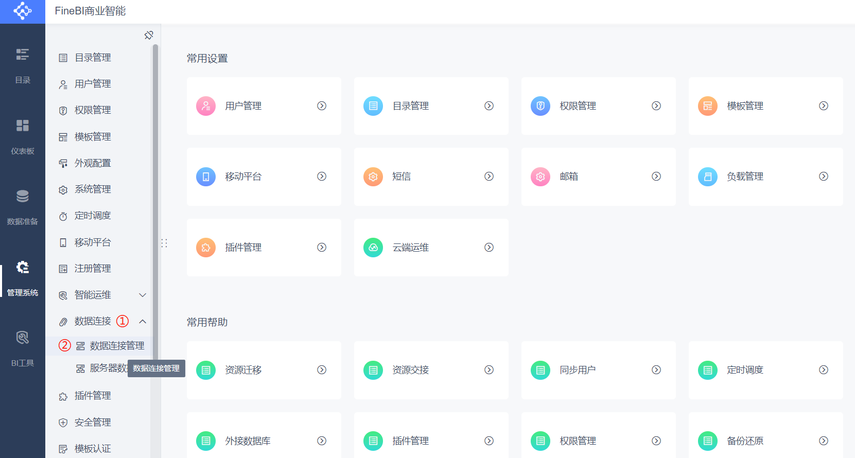
On the right side of the page, select [Driver Management] → [New Driver]

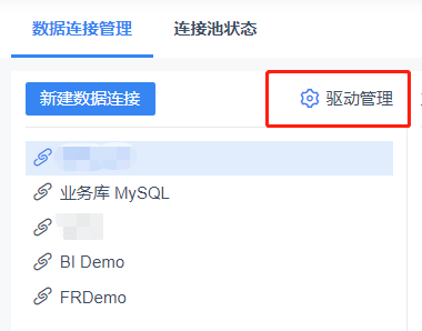
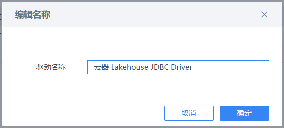
The driver name can be customized.

Upload the file at position ① in the picture, and after the file is uploaded and parsed, select the class at position ③ in ②.

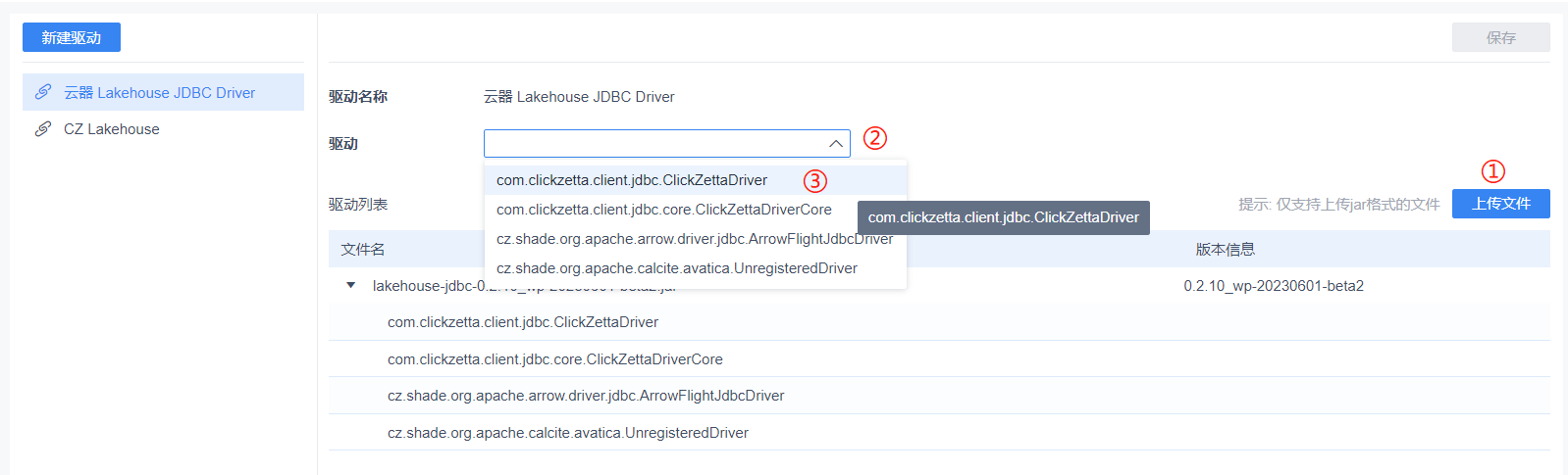
Click the top right corner to save the driver.

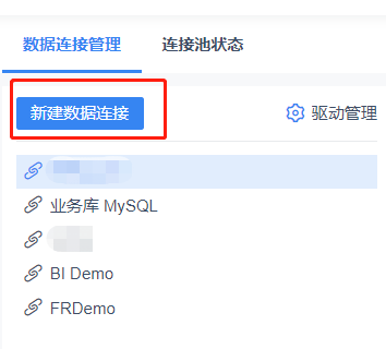
After the configuration is complete, we return to data connection management and can create a new Lakehouse data source.

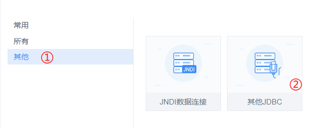
Since we are currently still a third-party connection driver, we choose [Other] → [Other JDBC]

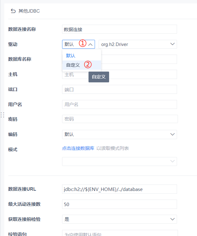
Here, we select [Custom] in the driver type.

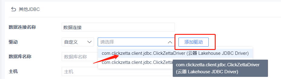
If we can find the driver option we just added, select it directly. If not, click [Add Driver] on the right.

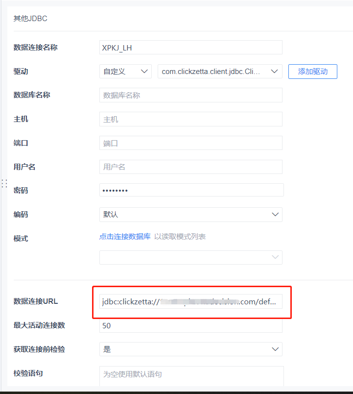
We only need to define a [Database Name], and fill in [Username], [Password], [Data Connection URL], etc. If you are not sure how to fill in the URL, you can check the SDK section of the help documentation or contact your account manager.

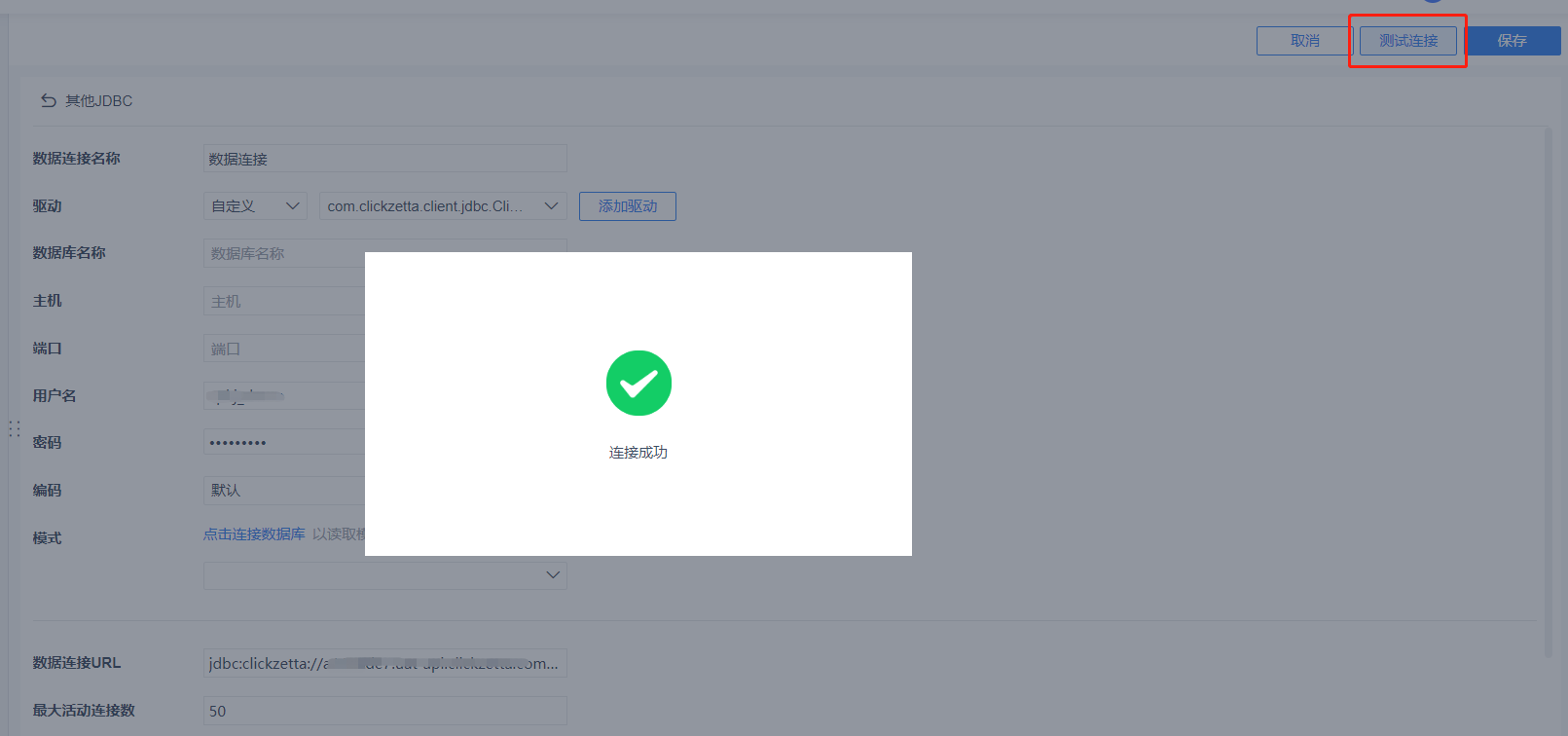
After filling in, click [Test Connection]. If the configuration is correct, it will display "Connection Successful". Click the [Save] button to complete the creation.

If the connection name is affected by the URL, you can also customize it by [Renaming].

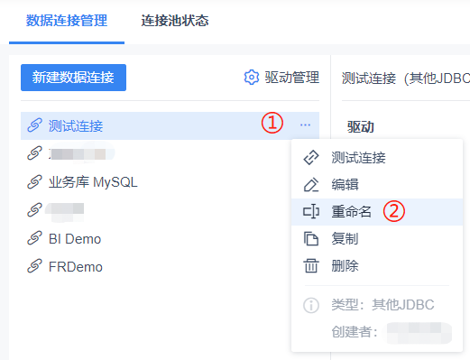
After the data connection is successfully created, the BI tool can access Singdata Lakehouse just like accessing other databases. Create datasets based on the data source, add database tables, and you can access the tables in Lakehouse.

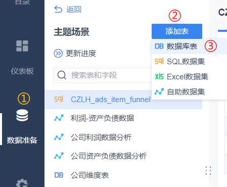
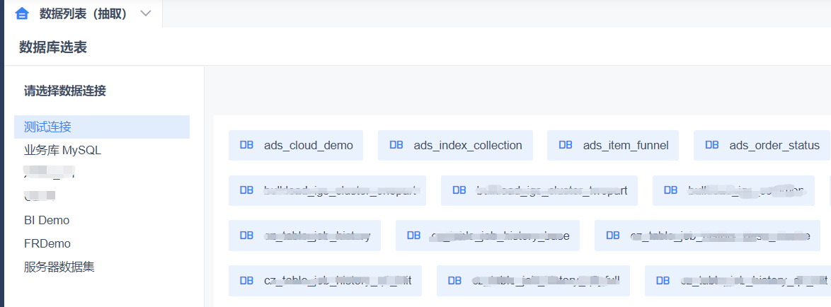
Create a dashboard to reference the dataset for arrangement. Interested users can refer to the FanRuan BI help documentation. https://help.fanruan.com/finebi/

Through certain dashboard style designs, we can create colorful BI dashboards. The following images are demo examples based on mock data