Analytical Cluster Planning, Configuration, and Best Practices

Analytical Scenario Requirements

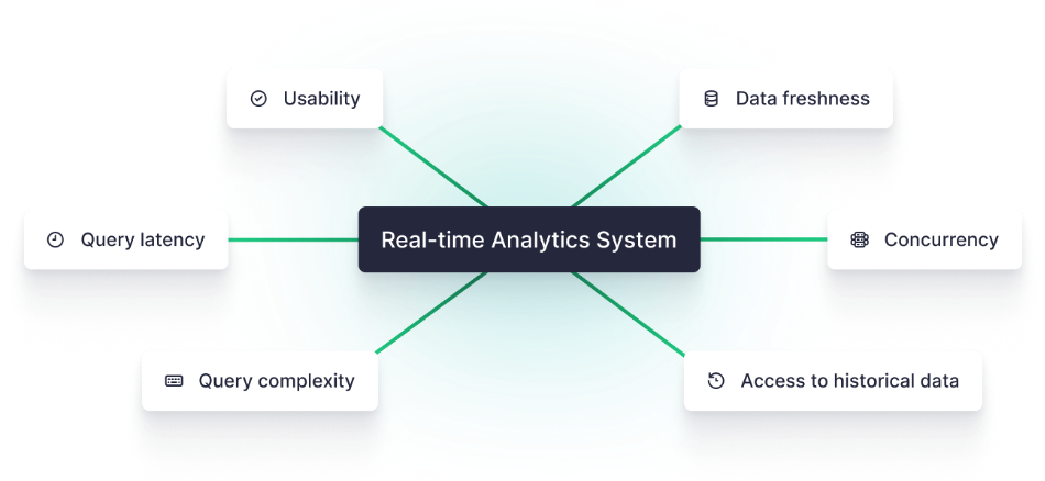
•Data Freshness: Real-time collection and processing of rapidly changing data

•Low Latency Queries: Provide second-level, sub-second query latency to ensure SLA

•Support for Complex Queries: Meet the analytical requirements of different business logics and data scales

•High Concurrency: Multi-concurrency for end users

•Historical Detail Queries: Support real-time historical comparison, historical retrieval, and exploratory analysis at the detail level

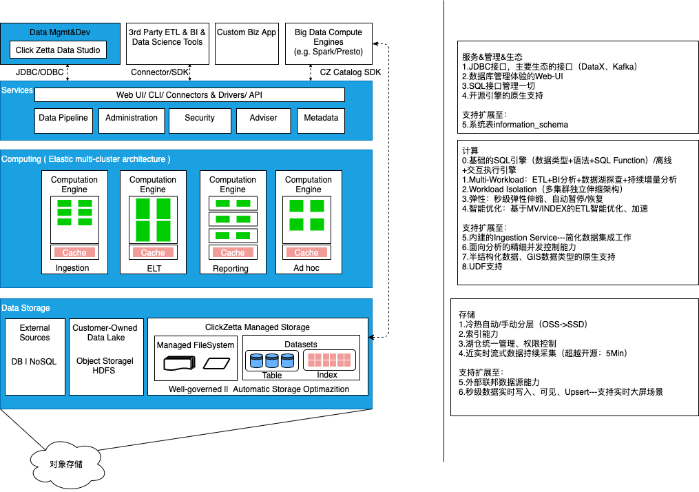
Singdata Lakehouse Product Capabilities in Analytical Scenarios

Category	Product Capability	Applicable Scenarios
Storage	Columnar Storage	Most ETL, OLAP analytical scenarios
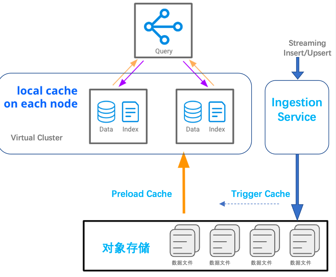
	Local Cache	Local Cache is provided by the local SSD of the computing resource Virtual Cluster, accelerating data I/O
	Cache Strategy: LRU, Preload Cache	LRU: Automatically cache hot data based on Query identification Preload Cache: Incrementally cache new data proactively based on a fixed range of data objects set by analysts, ensuring SLA
Data Layout	Partition	Large-scale tables with continuous time-based writes
	Bucketing + System Compaction Service automatically re-clustering to maintain new data bucketing aggregation	Commonly used in ETL+BI scenarios for filtering based on cluster key conditions
	SORT	Improve the efficiency of sort key condition filtering, commonly used in BI analysis scenarios
	Lightweight Index: bloomfilter index	Specify key point check filtering, can be used in combination with Cluster key, commonly used in BI analysis scenarios
Import/Export	COPY command	Batch export and import based on file method
	Real-time Ingestion Service	Provides real-time write API, supports Append/Upsert real-time writing, aimed at scenarios requiring data freshness
Compute	CZ SQL Engine provides two different load-optimized execution modes: ETL DAG execution optimization, MPP+Pipeline analysis execution optimization mode	Differentiated use through different types of Virtual Clusters: General Purpose, Analytics
User Interface	Studio Web-UI	Ad-hoc analysis, data processing tasks
	JDBC	Connects to a wide range of BI/client tool ecosystems
	SQL Alchemy/Java SDK/Go SDK	Python, Java, Go programming interfaces

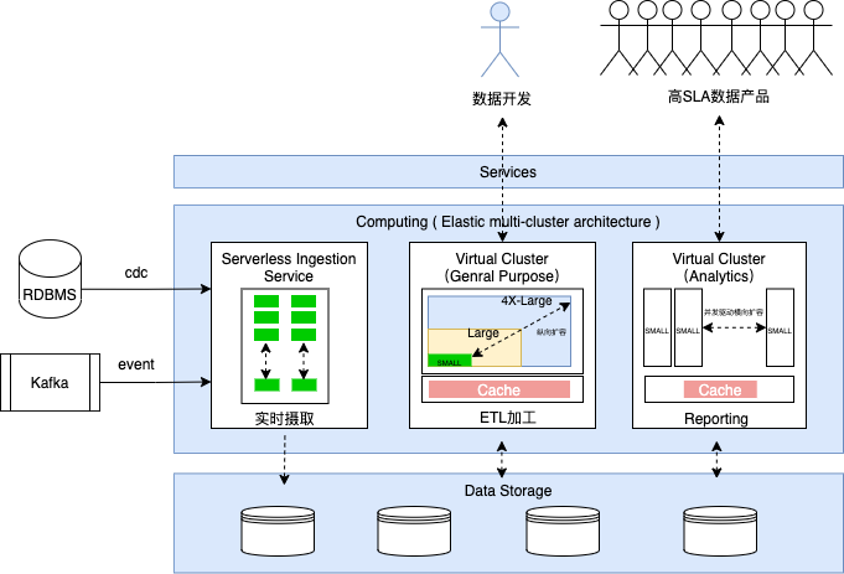
Reasonable Planning and Use of Virtual Cluster

<Notes>

This chapter will introduce the product features and planning methods for using ClickZetta Lakehouse's elastic computing resources.

Introduction to Virtual Cluster Features

<Notes> ## Compute Cluster (Virtual Cluster, VC) <a name="compute-cluster"></a>

The Compute Cluster (Virtual Cluster, VC) is a compute resource cluster service provided by ClickZetta Lakehouse. The compute cluster provides the necessary resources such as CPU, memory, and local temporary storage (SSD medium) to execute query analysis in the Lakehouse. These three resources are bundled into a compute scale unit called the Lakehouse Compute Unit. CRU serves as an abstract, standardized measurement unit for the size and performance of compute resources.

ClickZetta Lakehouse measures the actual usage duration of different specifications of compute resources (measured in seconds), and the different specifications of CUR and their unit prices are as follows:

Lakehouse Virtual Cluster Specification	CRU	MAX_CONCURRENCY Default Value
X-Small	1	8
Small	2	8
Medium	4	8
Large	8	8
X-Large	16	8
2X-Large	32	8
3X-Large	64	8
4X-Large	128	8
5X-Large	256	8

ClickZetta Lakehouse supports elastic scaling of compute resources in two dimensions:

Vertical: Adjust the number of CRUs by modifying the size of the Virtual Cluster to increase or decrease the computing power and performance of the specified cluster.
Horizontal: Adjust the concurrency query capability by modifying the number of cluster replicas to expand or reduce the number of Cluster replicas.

Plan the Number and Size of Compute Resources Based on Load

Best Practices for Using Compute Resources

Achieve load isolation through multiple compute resources
- Use multiple independent Virtual Clusters to support different workloads. Create different compute resources and allocate them to different users or applications based on different needs such as periodic ETL, online business reports, and analyst data analysis to avoid SLA degradation caused by resource contention among different businesses or personnel.
Set automatic pause duration reasonably
- The compute resources of Lakehouse have the characteristics of automatically pausing when idle, automatically resuming when a job is initiated, and billing based on the actual resource usage duration (not billing during the pause phase). This can be set through the AUTO_SUSPEND_IN_SECOND parameter, with a default of automatically pausing after 600 seconds of no queries.
- Recommendations for different scenarios (considering data cache and resource resume time in two dimensions)
  - For low-frequency Ad-hoc queries or ETL jobs, set AUTO_SUSPEND_IN_SECOND to around 1 minute.
  - For high-frequency analysis scenarios, set AUTO_SUSPEND_IN_SECOND to 10 minutes or more to keep the data relied on by the analysis always in the cache and avoid the latency degradation caused by frequent VC start and stop.
Choose the resource type of the Virtual Cluster based on the load type
- General Engine (VCLUSTER_TYPE=GENERAL) can complete all the tasks done by the analysis engine when the requirements for concurrency and job timeliness in analysis scenarios are not strong. It is optimized for batch processing workloads, prioritizes throughput, supports resource contention & sharing, and is suitable for ELT, data import (such as external table reading and writing), and Ad-hoc queries.
- Analytics Engine (VCLUSTER_TYPE=ANALYTICS) supports an analysis engine with a specified number of job concurrency. It is suitable for scenarios with strong guarantees on query latency and concurrency capabilities, such as reporting, dashboards, and critical business data products.
Use elastic concurrency capabilities to support critical data applications
The analytical Virtual Cluster supports multiple Replica features, with the default number of Replicas being 1. This can be modified during or after creation. Each Replica supports a specific query concurrency (determined by the MAX_CONCURRENCY parameter, which defaults to 8). The total concurrency supported by each Virtual Cluster is: Replica Number * MAX_CONCURRENCY
Preview
- Concurrency settings: Increasing concurrency may reduce the query performance of a single query when the size of the Virtual Cluster is fixed. In most cases, it is recommended that the concurrency limit does not exceed 100. The concurrency value is recommended to be a multiple of 8. An example is as follows:


--Create an analytical VC, enable elastic concurrency (min_replicas=1 max_replicas=3)
create vcluster if not exists your_ap_vc vcluster_size='XSMALL' vcluster_type='Analytics'  AUTO_RESUME=TRUE AUTO_SUSPEND_IN_SECOND=300 min_replicas=1 max_replicas=3 ;
—Modify the replicas parameter to increase the number of horizontal scaling replicas to enhance elastic concurrency
alter vcluster your_ap_vc set max_replicas=6;
--Modify the concurrency size of a single replica, suitable for fixed report scenarios with simple calculation logic and small data scale
alter vcluster your_ap_vc set MAX_CONCURRENCY=32 ;
--Modify the specification size of the Virtual Cluster, affecting the specification concurrency of all elastic concurrency created replicas to improve the query performance of a single query
alter vcluster your_ap_vc set vcluster_type='MEDIUM';

3. Query and configure MAX_CONCURRENCY
- Query MAX_CONCURRENCY
Use the following statement to query the configuration parameters of the specified VC, where you can find the current MAX_CONCURRENCY configuration value of the VC cluster:
DESC VCluster <name>
- Configure MAX_CONCURRENCY
Use the following statement to configure the MAX_CONCURRENCY of the specified VC. For analytical VC clusters, the MAX_CONCURRENCY configuration applies to all instances within it.
ALTER VCluster <name> SET MAX_CONCURRENCY = {desired positive integer}

Lakehouse Virtual Cluster Capacity Design Recommendations for Different Scenarios

The main business characteristics of the current ClickZetta Lakehouse supported business scenarios are as follows:

Scenario/Workload	Scenario Requirements	Resource Requirements	Data Scale and Query Latency Requirements	Query Characteristics	Concurrency Characteristics
Fixed Reports	High concurrency, stable low latency	Small + Elastic Scaling	• Small, query GB scale • TP95 <3 seconds	Simple logic, fixed pattern on processed data	For a wide range of frontline personnel, 10~100 or more
Ad-hoc	Detailed data supports interactive exploration and analysis	Medium	• Medium, 100GB~10TB • Most queries expected within 10 seconds, tolerant of complex query latency	Relatively complex logic	For professional analysts, fewer (related to organization size)
ETL	Stable output as planned, cost-sensitive, elastic demand under burst situations (e.g., data replenishment, temporary output)	Large	• Large, TB~PB+ level • Hourly level, SLA requirement for output completion time	Complex logic, processing type: many inputs and outputs	Low, multi-tasking for single user, accepts job queuing

Virtual Cluster Resource Specification Reference

This document plans to provide sample resource specification designs from the dimensions of business load type, execution frequency, job concurrency, data processing scale, and SLA requirements for reference.

Load Type: Includes ETL, Ad-hoc, Reporting, real-time analysis (Operational Analytics, etc.) with different data warehouse workload characteristics
Execution Frequency: Execution cycle of related loads
Concurrency: Number of jobs to be executed simultaneously
Data Processing Scale: Average data volume scanned per job
Job Latency SLA: Expected task delivery time in business

Example:

Business Scenario	Load Type	Execution Frequency	Job Concurrency	Data Processing Scale	VCluster Type	Job Latency SLA	VCluster Name	VCluster Size
ETL Scheduling Jobs	Near real-time offline processing	Hourly	1	1 TB	General Purpose	15 Min	etl_vc_hourly	Medium
	T+1 Offline Processing	Daily	1	10 TB	General Purpose	4 Hours	etl_vc_daily	X-Large
Tableau/FineBI	Ad-Hoc Analytics	Ad hoc	8	1 TB	General Purpose	<1 MinTP90:<5s	analytics_vc	X-Large
数据应用产品	Applications	On demand	8	100 GB	Analytical	<3 seconds	application_vc	Medium
		On demand	96	100 MB	Analytical	<3 seconds	application_vc	Medium
ClickZetta Web-UI<数据开发测试>	Ad-Hoc Analytics	Ad hoc	8	3 TB	General-purpose	< 1 MinTP90:<15 s	analytics_vc(shared with Analyst BI exploration)	X-Large

Note: The above examples are for reference only. In actual business environments, resource planning should be based on the actual business results, as they are influenced by various factors such as query complexity, data model (partitioning, bucketing), and cache hit rate.

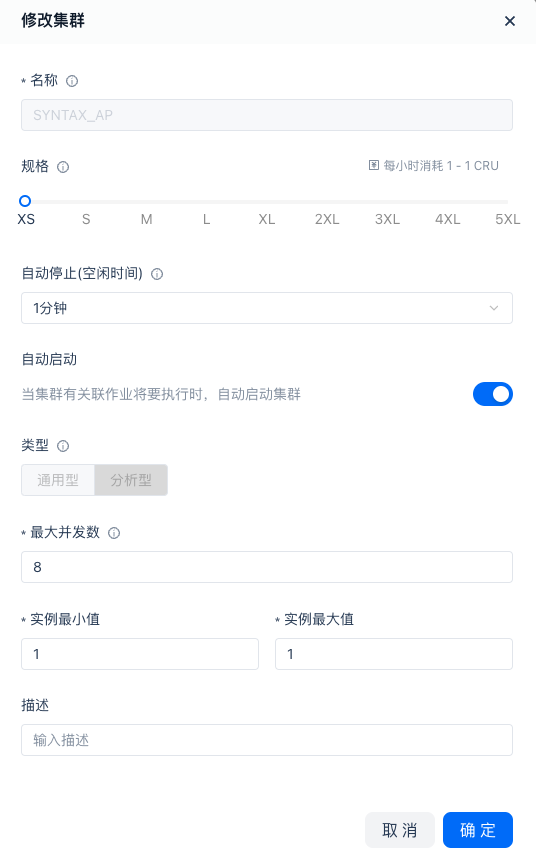
Configuration of Virtual Computing Resources Based on Concurrency Requirements

Singdata Lakehouse analytical virtual computing clusters (Virtual Cluster) are suitable for scenarios with high query latency requirements such as ad-hoc, multi-concurrent fixed reports, and real-time analysis. Analytical virtual computing clusters offer the following configuration options:

Configuration Options	Description
Specification	The size of the computing resource instance within the virtual cluster. The specification ranges from XS to 5XLarge, with each level increase doubling the computing resources.
Type	General-purpose or analytical, here we use analytical.
Maximum Concurrency	The number of concurrent queries supported by a single computing resource instance. When the maximum concurrency of a single instance is exceeded, new queries will queue or be allocated to other computing resource instances within the virtual cluster.
Minimum Instances	The number of cluster instances when the virtual cluster initially starts, default is 1.
Maximum Instances	The maximum number of instances that the virtual cluster can use. When the maximum instances > minimum instances, it means that new computing instances will be automatically scaled out based on whether the number of concurrent requests received by the virtual cluster exceeds the total maximum concurrency of all computing instances, until the current number of instances = maximum instances.
Current Instances	The number of instances currently used by the virtual cluster.

The following diagram describes the relationship between the parameters related to the analytical virtual cluster:

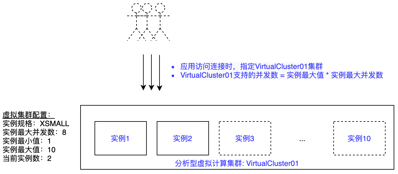
Vertical Scaling: The instance specification is an option for vertical scaling of the virtual cluster. Adjusting the instance specification can provide more computing power for a single job to improve job performance.

Horizontal Scaling: Elastic capability aimed at improving cluster concurrency. Analytical clusters are designed for horizontal scaling scenarios, providing a multi-instance architecture within a single cluster. Each analytical cluster sets the initial number of instances and the upper limit of horizontal scaling by setting the minimum and maximum instances.

In actual business scenarios, data products facing users often have SLA requirements, such as P99 query latency under 100 concurrency being less than 2 seconds. At the same time, it is hoped that computing resources are fully utilized to minimize resource costs while meeting business needs. As shown in the figure below:

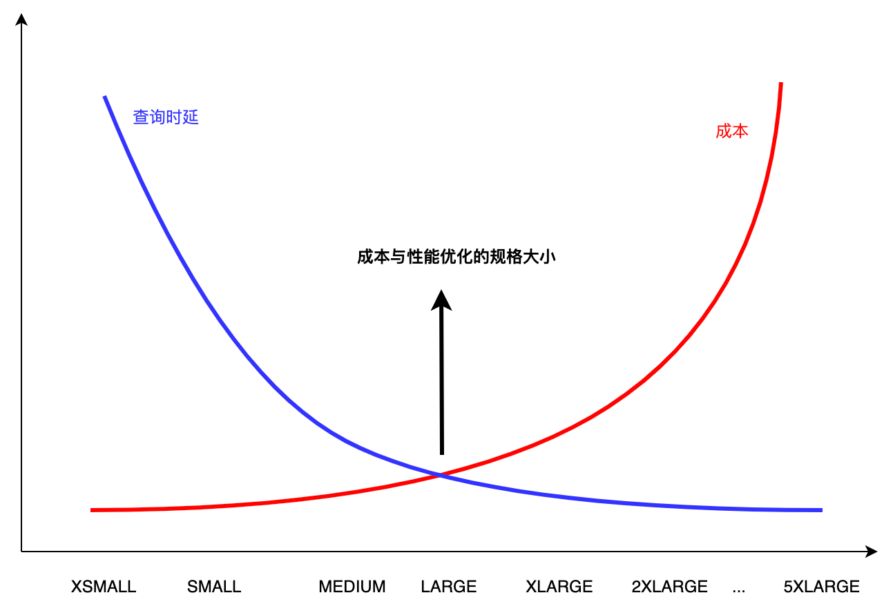
In specific business scenarios, we hope to find the minimum resource requirements that meet the SLA performance requirements. This article, from a practical perspective, combines example scenarios to determine reasonable resource specification configurations through the following steps.

Scenario Example

The data processed by the data platform is packaged as data products (such as Dashboards), supporting up to 20 concurrent user queries externally. Each user request for a data product generates an average of 8 data platform queries (an average of 8 metrics per Dashboard), which translates to 160 concurrent queries on the data platform. The requirement is that P99 query latency should be less than 1.5 seconds.

Data queries have the following characteristics:

Dataset size for Dashboard queries: around 1GB.
Characteristics of Dashboard queries: mainly point queries, filtering, and aggregation, without JOINs.

This document uses the SSB FLAG 1G dataset and query statements to simulate the above scenario, to verify the cluster configuration and performance under concurrent queries.

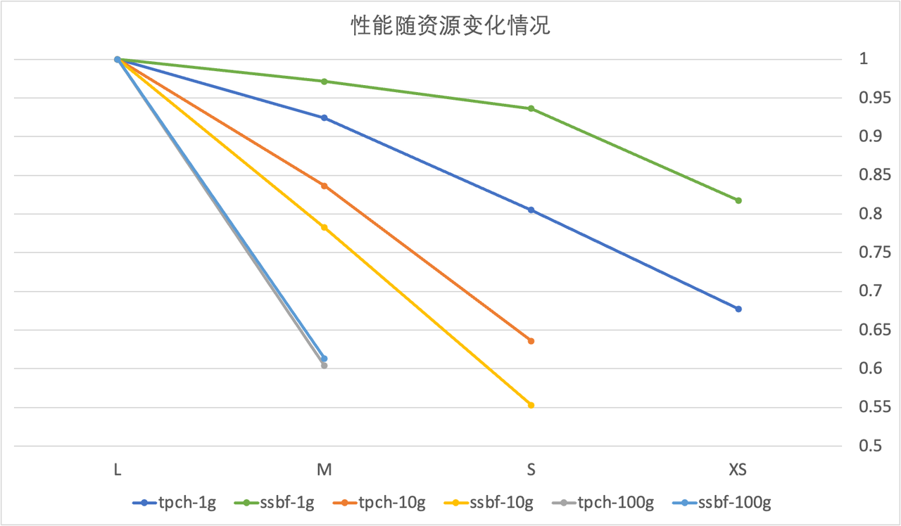
Step 1: Find the single instance specification size that balances performance and cost

Run queries using clusters of different sizes (this document tests several sizes from Large to XSMALL) to find the smallest resource specification that does not significantly degrade performance.

As shown in the figure below, the SSBF-1G benchmark maintains over 80% of the performance of the Large specification even at the XSMALL specification. Here, the XSMALL specification is chosen to support data products.

Note: Based on test results, it is recommended to use Large size for 100G data scale by default, Medium for 10G, and Small or XSmall for 1G.

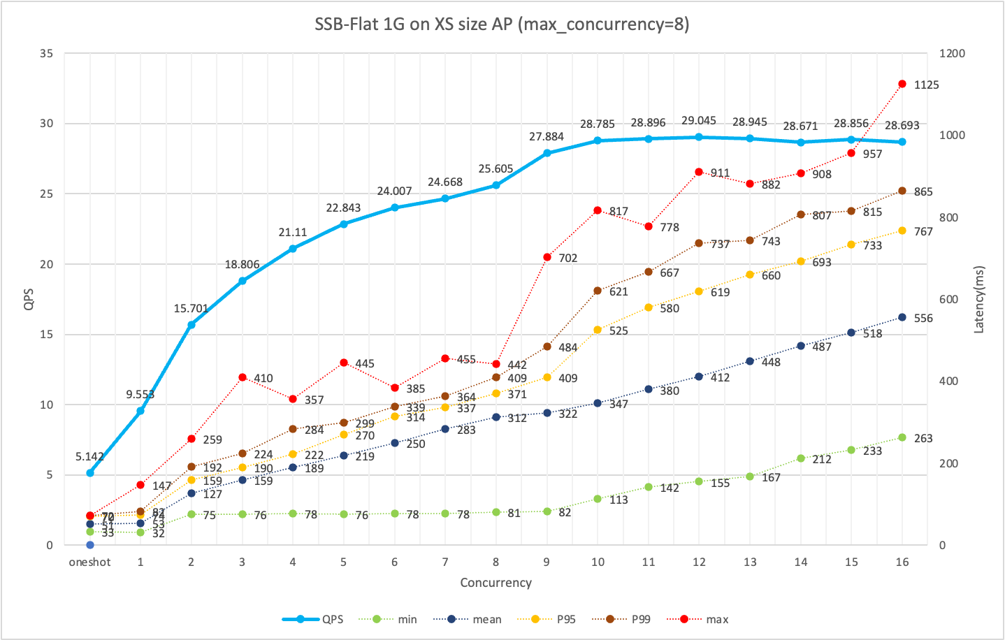
Step 2: Test the query SLA and QPS under different levels of concurrency for a single instance

As shown in the figure below, using an XSMALL specification cluster, at 8 concurrent requests, the QPS is high, and the P95/P99 query performance is good.

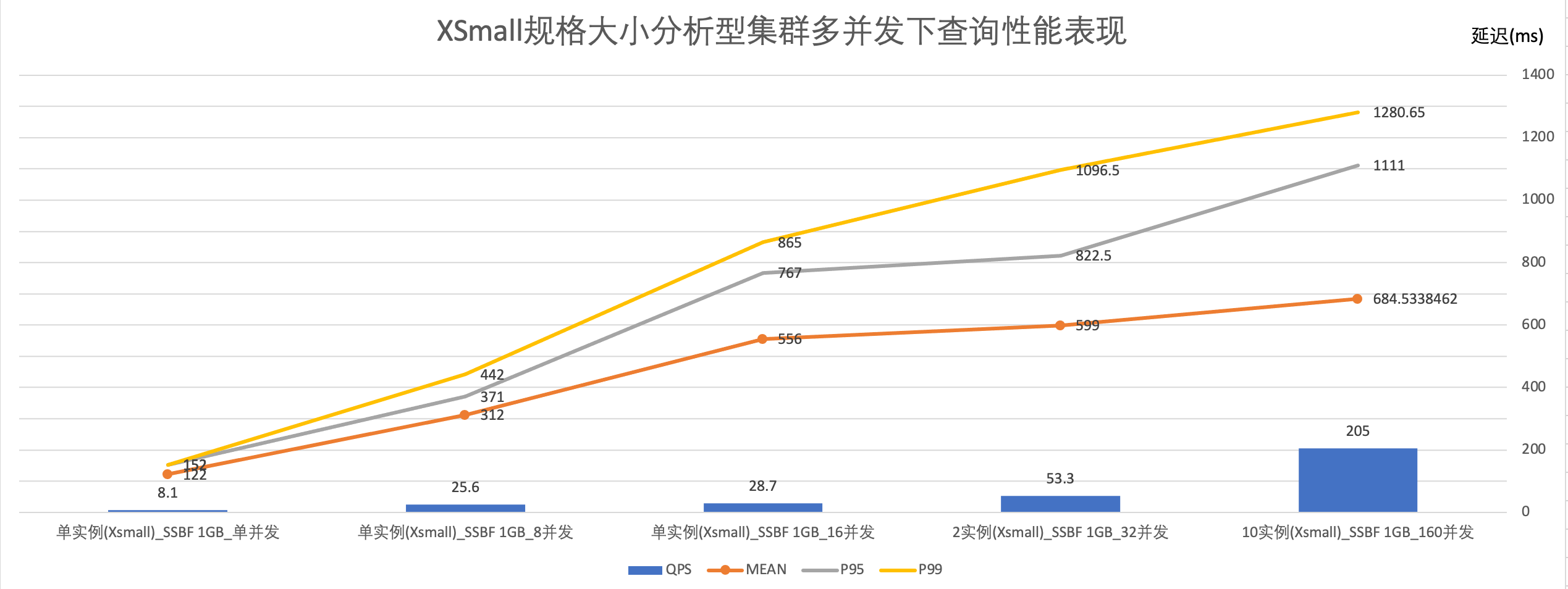
Step 3: Find the maximum number of instances that meet both the SLA and actual business concurrency needs through horizontal scaling

As introduced earlier, the number of concurrent queries a cluster can support = maximum number of instances * maximum concurrency per instance. In principle, once the single instance specification size is determined, horizontally scaled instances should have the same query SLA and QPS.

Based on the test data, this document uses an XSMALL specification, with a maximum of 10 instances in a virtual cluster, to meet the need for 160 concurrent queries. The query response time P95=1111 milliseconds, P99=1280.65 milliseconds.

Summary

This section uses a small-scale dataset with simple concurrent query scenarios to illustrate how to reasonably set the virtual compute cluster specifications and related parameters of Singdata Lakehouse to meet SLA requirements.

To simplify this reference process, some empirical values are provided below based on test information for reference.

Load Type	Data Scale	VC Instance SIZE	Single Instance QPS Reference	Scenario Example
Fixed Reports/Serving Queries (mainly simple filtering or aggregation)	1GB	XSmall	25	Demand Example: 1. Result data scale is 10GB 2. Query analysis is simple filtering or aggregation 3. SLA requires support for 200 concurrent queries 4. Average response time: 1 second Cluster configuration example: 1. Analytical VC, SIZE choose Medium specification 2. Based on a single Medium having 20 QPS for simple queries on 10GB data, it is estimated that 10 instances can provide 200 QPS, so the maximum number of instances is set to 10.
	10GB	Medium	20
	100GB	Large	<10
Ad-hoc/BI dynamic report generation (with associative analysis, complex calculations)	1GB	Small	15
	1GB	Medium	25
	100GB	XLarge	<10

Improve the Stability of Key Business Queries Using Preload Cache Mechanism

Preload Working Mechanism and Applicable Scenarios

Suitable Usage Scenarios

• Cache existing data with computing resources proactively to avoid latency on the first access to historical data

• Trigger cache upon real-time data write-in to reduce query latency jitter after new data is written to disk

Usage Method

Set the data object range for PRELOAD for specified computing resources, supporting enumeration and wildcard methods.


-- Set the data objects to PRELOAD when creating the compute cluster

create vcluster if not exists <name>

auto_preload_in_second=600

PRELOAD_TABLES="s1.t1,s1.t2";

-- Modify the compute cluster to add or modify PRELOAD data objects

ALTER VCLUSTER <name> SET PRELOAD_TABLES='schema01.tb01,schema01.tb02,schema01.tb03';

View the current Preload configuration of computing resources:

Preload eliminates query jitter for new data in real-time analysis scenarios

Uncached file ratio	TPCH 100G (0%)	TPCH 100G (1%)	TPCH 100G (5%)	TPCH 100G (10%)	TPCH 100G (20%)	TPCH 100G (30%)
Query latency	9300 ms	15418ms	20311ms	19027ms	18815ms	20841ms

Computing Resources and Job Monitoring

Computing Resource Status

Monitoring via Web-UI

Monitoring via SQL API


desc vcluster quning_ap_vc;

name	QUNING_AP_VC
creator	demo_project
created_time	2024-01-28 23:15:13.625
last_modified_time	2024-03-27 09:59:48.212
comment
vcluster_size	XSMALL
vcluster_type	ANALYTICS
state	RUNNING
scaling_policy	STANDARD
min_replicas	1
max_replicas	4
preload_tables	qn_demo.lineitem,upserted_ssb_1g.lineorder_flat,leanken_preload.*
current_replicas	1
max_concurrency_per_replica	8
auto_resume	true
auto_suspend_in_second	1800
running_jobs	0
queued_jobs	0
query_runtime_limit_in_second	259200
error_message

Job Monitoring

Scenario: Job failure, long-running jobs, monitoring jobs for specific users/VC, job runtime and cost statistics, monitoring specific TAGs.

Monitoring through Web-UI

Add filter conditions: such as filtering specific jobs/job groups by TAG


--Session级别设置query_tag
set query_tag='aa';
select 1;

Monitor Recent Job Execution Success/Queue/Long Running Status via SHOW JOBS Command

The SHOW JOBS command retrieves ongoing and recently completed jobs within the workspace's computing resources.


SHOW  JOBS  [IN VCLUSTER vc_name] [WHERE where_condition ] [LIMIT num];

Note:

List the most recently executed jobs, including both completed and running jobs. Users can use this command to list jobs they have permission for. By default, it displays tasks submitted in the last 7 days, with a maximum query limit of 10,000 entries.


-- View the recent job history within the Workspace
show jobs limit 100;

-- Filter by conditions: view jobs with specified computing resources, submitted by a specific user, and with execution time exceeding a certain duration
show jobs where vcluster_name='quning_ap_vc'  
and creator='demo_project' and (end_time - start_time) > interval 0.1 second  
limit 100;

name	QUNING_AP_VC
creator	demo_project
created_time	2024-01-28 23:15:13.625
last_modified_time	2024-03-27 09:59:48.212
comment
vcluster_size	XSMALL
vcluster_type	ANALYTICS
state	RUNNING
scaling_policy	STANDARD
min_replicas	1
max_replicas	4
preload_tables	qn_demo.lineitem,upserted_ssb_1g.lineorder_flat,leanken_preload.*
current_replicas	1
max_concurrency_per_replica	8
auto_resume	true
auto_suspend_in_second	1800
running_jobs	0
queued_jobs	0
query_runtime_limit_in_second	259200
error_message

View Historical Execution Jobs through INFORMATION_SCHEMA

The data dictionary view of INFORMATION_SCHEMA has a delay of about 10 minutes, which is suitable for analyzing long-term historical job data. For online real-time job analysis, use the SHOW JOBS command to obtain it.


-- View job history in the current workspace
select * from information_schema.job_history limit 100;

-- View job history in the current Lakehouse service instance
select * from sys.information_schema.job_history limit 100;